Bench instrument software
RF Bench Analyser
A full spectrum analyser front panel for the instruments on your bench. It began as one for a Rohde & Schwarz CMU200 or CRTU, and it now drives fourteen kinds of instrument, from that radio tester to a tinySA, an oscilloscope, a NanoVNA and a rack of SDRs: seven traces, eight markers, fourteen measurement windows with a network analyser and a transmitter and receiver test bench among them, level calibration, limit masks, scripting in C# or Python, and an unattended watch that keeps the sweeps around whatever it caught.
$9.99 when it lands. One purchase, no subscription, no licence server, and it keeps working offline.
A very good instrument with a very small screen
The CMU200 is a superb piece of test gear that turns up second hand for a fraction of what a spectrum analyser costs, and it can genuinely sweep 10 MHz to 2.7 GHz. What it does not have is a spectrum analyser’s front panel. Everything is behind a menu tree on a small screen, and the good measurements are the ones nobody finds.
So this started as the front panel. The instrument does the RF; the PC does the traces, the markers, the maths, the logging and the pictures. Then the rest of the bench wanted the same front panel: the tinySA, the oscilloscope, the SDR receivers, the transmitters and the NanoVNA. Each one now sits behind the same window, and two of them together make a bench: one keyed into the other through a cable, and measured.
It is not free software and it is not open source. It will be $9.99 on the Microsoft Store, which it is not on yet: one purchase, no subscription, no licence key to lose, and no phoning home. What you get for that is roughly two years of evenings and a program that has been driven against real instruments until it stopped lying.
It is written honestly about what it knows. Where a number has been checked against a real instrument, it says so. Where it has not, it says that too, on the screen, in the handbook and below on this page. An analyser that quietly reports a plausible wrong answer is worse than one that admits it cannot tell.
📈 One work surface
The plot takes the whole window. Settings float over it and get out of the way, and every measurement that needs room gets a window of its own.

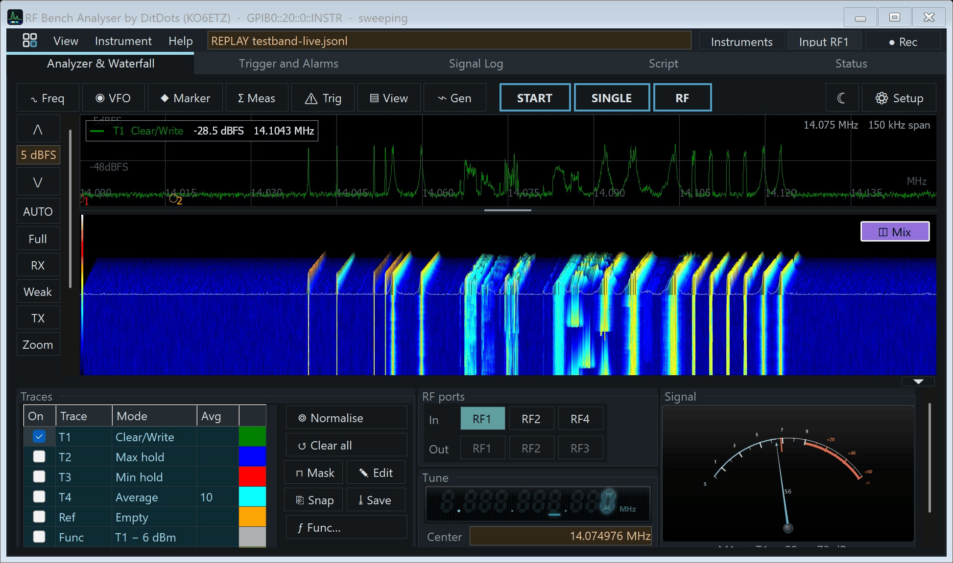
Main window, 3-D waterfall: a minute of the live 20 m test band, 5120 points across 150 kHz, in the dark theme: the trace on top, the terrain waterfall under it, and the trace table, RF ports, tuning and signal meter along the bottom.

A panel over the trace: the Markers panel open over the plot, a normal and a delta marker reading level and offset. Settings reach you without costing the trace any width.

Light theme: the same band in the light palette, for a bright room.

The VFO panel: the current frequency in large figures, a keypad and a knob to move it, a Listen row that demodulates at the VFO, and ten memories.

The command launcher: every menu item as a tile, grouped as the menus are, with a box at the top to type the name of a command.
🔢 The shape of it
What the instruments give you, and what the software makes of it.
📡 The instruments it drives
Every instrument describes itself to the window: its range, its connectors, its bandwidths, its generator if it has one. The window builds its controls from that, so nothing offers a setting the instrument cannot take.
| Instrument | Reached over | What it is here | On real hardware |
|---|---|---|---|
| R&S CMU200, CRTU, CMU 300 | GPIB, through VISA | Swept analyser, 10 MHz to 2.7 GHz; its own generator; its counter and power meter; the CMU-B41 audio option | Yes, a CMU 300 |
| tinySA Ultra | USB serial | Analyser, 100 kHz to 5.3 GHz, and its generator | Yes |
| tinySA (original) | USB serial | Analyser, 100 kHz to 960 MHz | Not yet: its figures are the documentation’s |
| Rigol DHO800 and DHO900 | The network | An oscilloscope as an FFT analyser, DC to 70 MHz (100 MHz on the faster models) | Yes, a DHO804 |
| OWON DGE2000 | USB, through VISA | A signal source to 70 MHz, with its modulations and its own sweep | Yes, a DGE2070 |
| A PC sound card | Windows audio | A line or microphone input, a receiver’s I/Q, or the PC’s own sound output | Yes |
| Malahit DSP | Its I/Q over USB audio, tuned over its own CAT port | Receiver, 10 kHz to 2 GHz | Yes |
| RTL-SDR | rtl_tcp, on this PC or the network | Receiver, 24 MHz to 1.766 GHz, and direct sampling below 14.4 MHz | Yes, a Blog V4 and a generic stick |
| HackRF One | USB, through libhackrf | Receiver and transmitter, 1 MHz to 6 GHz, with its firmware’s own fast sweep | Yes, keyed into the CMU 300 |
| Ettus USRP B210 and compatibles | USB, through the ShackLinkUsrp helper | Receiver and transmitter, 70 MHz to 6 GHz, on all four sockets | Yes, two boards, both keyed |
| ADALM-Pluto and Pluto-class boards | USB or Ethernet, through the same helper | Receiver and transmitter, 70 MHz to 6 GHz | Yes, keyed into the CMU 300 |
| Hermes Lite 2 | The network, openHPSDR Protocol 1 | Receiver, 10 kHz to 38.4 MHz, a wideband view, and its HF transmitter | Yes, keyed into the CMU 300 |
| SDRplay RSP | USB, through SDRplay’s own API | Receiver, 1 kHz to 2 GHz | Yes, an RSP1 clone |
| NanoVNA-H family | USB serial | A vector network analyser, 10 kHz to 1.5 GHz; and its output as a signal source | Yes, a NanoVNA-H 4 |
| A SigMF recording | A file | Played in a loop as though it were the instrument that made it | Not an instrument |
Your transceiver
Through OmniRig or Hamlib’s rigctld, a rig’s knob moves the sweep and a click on a signal tunes the rig. As a device under test it is keyed by CAT, a serial line or by hand, and never past its time-out.
An input switch
A relay board in front of the analyser’s input, so the antenna, the generator or the device under test is picked from the window. Up to sixteen inputs, over Wi-Fi or USB.
Another PC
Run a relay on the PC the instruments are plugged into and drive them from a window anywhere on the network. Only the connection crosses it; a recording made that way is the same as one made beside the instrument.
🤝 Two instruments make a bench
One instrument is the analyser and another can be the source: a HackRF beside a CMU200, an OWON generator beside the oscilloscope, a Pluto beside a tinySA. The instrument list draws the bench as two boxes with their connectors and the cables, pads and switch between them, and every measurement that needs a stimulus uses the source you set.

The bench, drawn: the instrument list, and under it the source, an antenna switch with six inputs, the pads and the analyser, each connector named as the instrument names it.
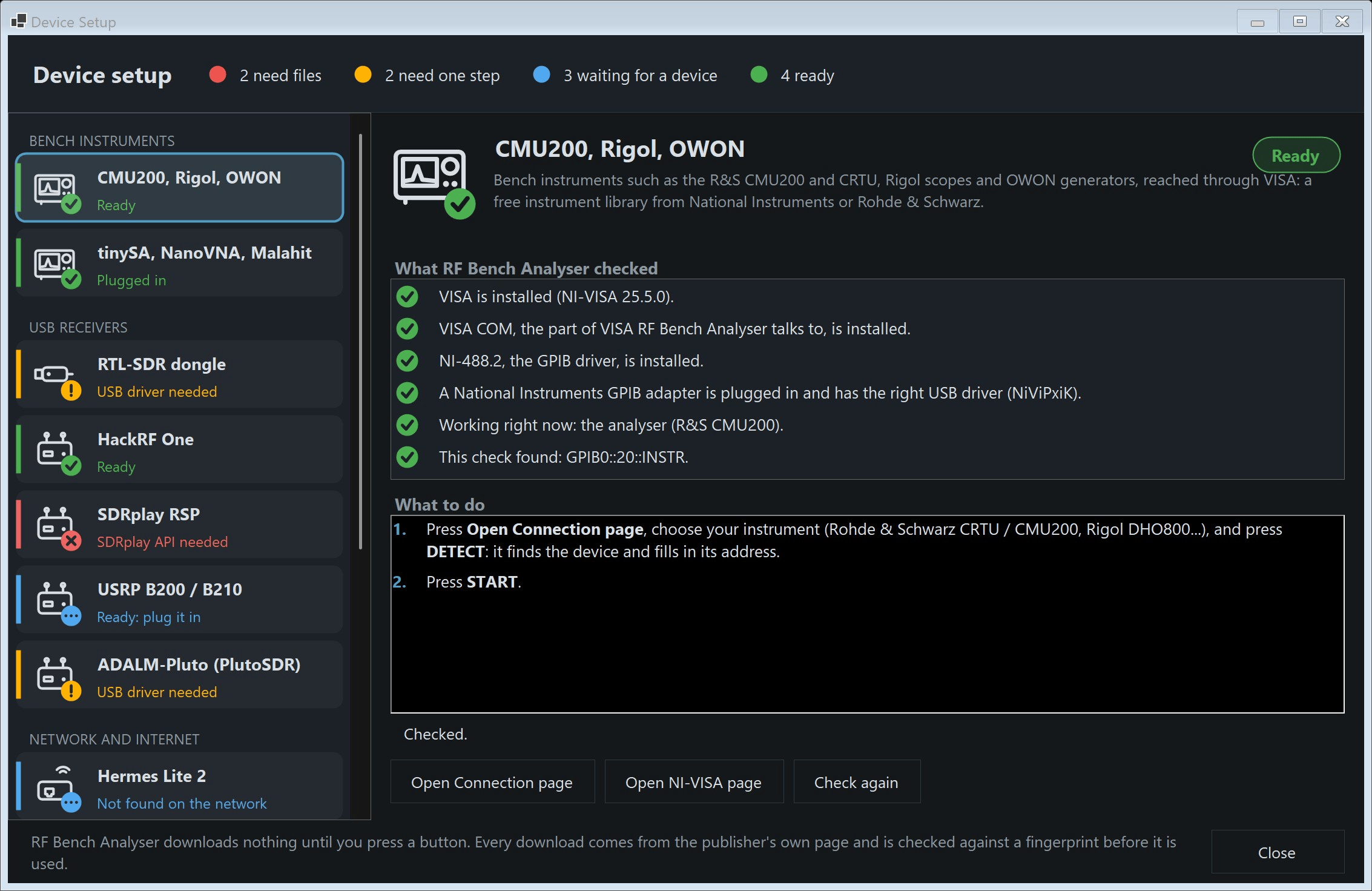
Device Setup: is this PC ready for each kind of instrument? What is installed, what Windows sees, what works right now, and the step that fixes what does not.
⚙️ What it does
The analyser itself: everything below works on whichever instrument is active.
📡 Seven traces, any of them anything
A table with a row per trace: on, name, mode, average count, colour. The four accumulating traces are interchangeable, so any of them can be clear/write, max hold, min hold, average or RMS, with its own average count. Two on Average with different counts is a perfectly ordinary thing to ask for.
Beside them sit a frozen reference, a loaded overlay from a file, and a computed function trace, with the last ten traces kept as snapshots you can lay over the live one.
➕ Thirteen trace functions
Difference, sum, combine, remove, deviation, envelope, floor, mean, relative to peak, noise density, smooth, ripple and VSWR, each shown in the picker with its formula.
Anything that combines two levels does it in the power domain and converts back, because the mean of two decibel readings is not the decibel of their mean power. A function of an unmeasured point stays unmeasured rather than becoming 0 dBm, which is the top of the scale.
◆ Eight markers that name their own trace
Normal, delta, band power and noise. A marker names which trace it reads, so one on max hold and one on the average can sit at the same frequency and disagree, which is what holding a max is for.
The peak search treats a flat top as one peak and reports its centre, which is what makes it work on modulated carriers rather than only on CW. Markers are remembered as frequencies, so they come back where you left them.
🎛️ A VFO, and you can listen to it
The current frequency is one number: a red line on the plot, a large readout, a keypad and a knob, and the centre of the sweep on a live run. A frequency is never typed into a box: every frequency field opens the same dialog, so a unit is always written.
On an instrument that hands over I/Q, the VFO panel’s Listen row demodulates AM, NFM, WFM, LSB, USB and CW at the VFO to the PC’s speakers, while the sweep carries on.
⏱ A frequency counter, twice
The trace counter fits a curve through the peak bin and its two neighbours. On a reference recording it finds a 14.040000 MHz beacon to within 0.06 Hz, where the bin it sits on is 17.8 Hz away. It says when it could not interpolate, because six decimals of a quantised number is worse than one that admits it.
Beside it, a key asks the instrument to count where it can, and the readout says how far the two are apart.
📋 A live table, and alarms on it
Fourteen measurement kinds, several at once, recomputed every sweep. A blank parameter means “work it out”, so a row gives you a number the moment you add it.
Any row can carry an alarm rule: a comparison, a threshold, and a dwell counted in sweeps rather than seconds, so a slower resolution bandwidth cannot change how long it takes to fire. A measurement that stopped succeeding is never read as “within limits”.
⚠️ Limit masks, including in dBc
Draw one on the plot in hertz and dBm, build one from a trace, or generate one from a template: a band edge, a spurious or harmonic limit, a two-tone IMD limit, an SSB splatter mask or an FM channel mask. Every saved mask appears as a tile drawn in its own shape, so you can see whether it belongs to this band at all.
A mask written in dBc is re-anchored every sweep to the carrier. With no usable anchor it reports NOT TESTED rather than testing against noise, and whatever is outside the mask is drawn on the plot in the alarm colour.
🔌 Signal generators, with a picture
Whichever instrument is the source: the CMU200’s own generator, a tinySA’s, a HackRF, a USRP, a Pluto, a Hermes Lite 2, a NanoVNA’s output or an OWON. Carrier, level, connector and the modulations that instrument offers: AM, FM, PM, SSB, DSB and pulse among them. The Gen key lights while the output is keyed, so whether something may be transmitting is visible from the trace.
Beside the boxes is a picture of the signal you have asked for, drawn as the analyser would draw it and labelled from the settings, not measured. A carrier sweep steps the output across a band, and draws itself against time.
🔬 Frequency response, with a stored calibration
A window that sets up, calibrates and runs a filter, duplexer or cavity measurement, with the generator and the analyser in one box or two. Points can be spread evenly, or concentrated where the skirts are: on a 150 kHz band that turns an even 112-point pass resolving 1.35 kHz into one resolving 100 Hz where it matters.
A through calibration can be stored to a file and reapplied, point for point, and is refused with a reason rather than stretched onto a grid it was not taken on.
⏲ Zero span
Park the sweep and the points become samples in time. Peak, average power, top, base, on/off ratio, burst count, pulse width, period, rate, duty cycle, rise and fall times, and droop.
Every average is taken in the power domain, crossings are interpolated, only complete bursts are measured, and anything the window cannot hold is reported as absent rather than guessed at.
🔧 Stitched sweeps, for real resolution
A band can be taken as up to 64 narrower sweeps, joined. On the CMU200, which returns 560 points whatever the span, that buys points and, more importantly, a narrower resolution bandwidth, because the instrument’s bandwidth floor rises with the span. On an SDR it is how a dongle that sees 2.4 MHz at a time sweeps the whole FM band.
On an FFT instrument a frame can be up to 32 768 bins. A seam has been checked against a carrier parked on it and lands within 0.03 of a bin.
💾 Recording, I/Q and video
Every sweep can be appended to a recording as it is drawn, and a recording replays through the whole application as though it were arriving from the instrument.
On an instrument that streams, the raw I/Q is recorded as SigMF, and a SigMF recording, this program’s or another’s, plays in a loop as an instrument you can sweep, zoom into and listen to. A key on the menu bar records the window itself as an MP4.
📜 Scripting in C# or Python, live
Write your own measurement against the traces and the markers, with every built-in measurement in scope, and run it once. Or switch on Live and it runs after every completed sweep, beside the trace it is measuring.
Python runs on your own CPython with numpy, and a script can read the raw I/Q the instrument is streaming. A run still going when the next sweep arrives skips that sweep rather than queueing, and the status line says how many.
🖥️ Instruments, profiles and presets
DETECT finds what is plugged in, on the bus, on USB and on the network, and keeps all of it, each with a name you give it. Switching instrument is one press, and the window rebuilds itself around the new one while it runs. Each instrument remembers its own band.
A profile is the whole application under a name, and a preset is a band. The amateur band plan is tinted on the plot and can be tuned from directly, through a converter in front of the instrument if there is one.
🗂️ Windows, or tabs
Every measurement window opens on its own and can go on a second monitor. Or tick View → Instrument Windows as Tabs and each one becomes a page of the main window instead, with the live sweep along its foot.
The Readouts window puts every number at once on another screen, and a command launcher shows the menus as tiles for a touch screen.
👁️ A status page that never bluffs
Two halves that are never mixed. On the left, what the application knows, with a column saying where each number came from: the frame that arrived, a box you typed in, or a model. On the right, what the instrument answers, with the command, the raw reply, and how long ago it was asked.
A reading older than the poll promises is dimmed, because a stale register that looks live is the whole failure mode of a page like this.
♿ Readable by a screen reader
Every entry box, readout, key and grid cell carries a spoken name that says what it is for, taken from a table rather than guessed from the nearest label. Several names carry the state too, because otherwise it exists only as pixels.
🔊 A USB knob as the VFO
A cheap USB volume knob tunes the sweep. A detent moves the VFO; a press walks the tuning step from 1 kHz to 10 MHz and wraps; the two extra buttons step the band presets. It is off by default and says why: while it is armed the volume keys are taken for the whole machine.
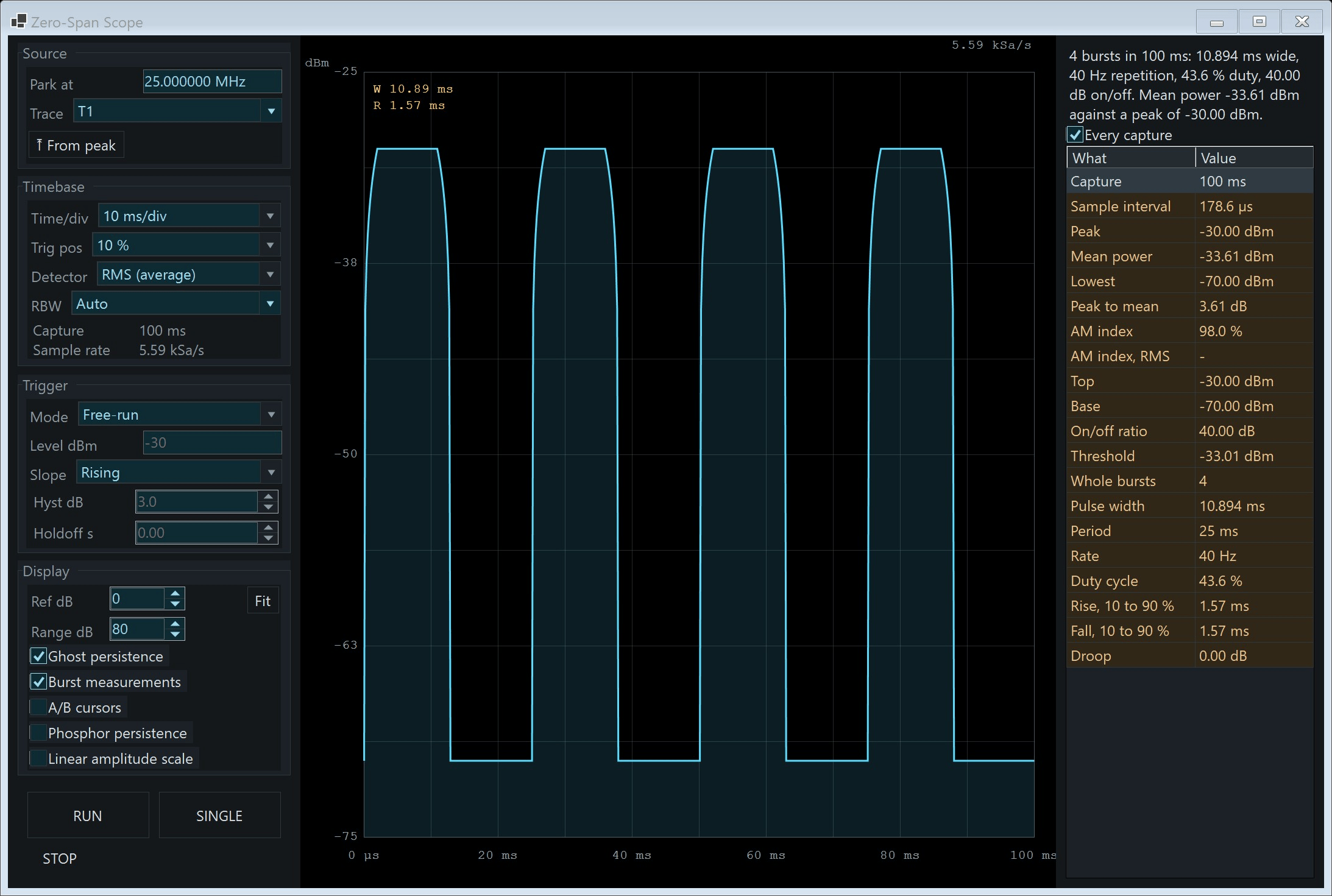
Zero span, a pulse train: parked at 25 MHz on the four-burst reference: width, period, rate, duty cycle and rise and fall times from one 100 ms capture.
📏 Measurement windows
A measurement that needs room gets a window of its own, with a large chart, its figures in words, and its data in and out as CSV. Every one says what it read and what it could not.
⚡ Power meter
An arc and a needle, the reading in dBm and in watts, and a chart of it against time: the instrument’s own power meter, a marker, a channel or the whole sweep. Declare the transmitter you are about to key and it is checked against the input’s rating, through the pad, before you key it.
🕑 Frequency stability
A frequency counted again and again: its error in hertz and ppm, the drift as the slope of a line fitted to the whole run rather than last less first, and the Allan deviation. Built for a transmitter warming up.
〰️ Modulation meter
FM deviation each way and RMS, AM depth, the modulating tone and a CTCSS tone, demodulated from the I/Q a receiver hands over. On the CMU200, which hands over none, it says where the same figures are instead: off the carrier’s sidebands.
🌊 Phase noise
L(f) in dBc/Hz, a decade at a time about the carrier, with the analyser’s own limit drawn beside it, so a curve that is really the analyser’s is never passed off as the transmitter’s. The integrated jitter, and a reference curve to compare against.
🎼 Two-tone test
Intermodulation against PEP and against a tone, which differ by 6 dB, so a figure is never quoted without saying which. The two tones come from your own source, the CMU-B41’s audio generator, or the bench’s generator, and the window says what to key.
📈 Gain compression
The generator stepped up at one frequency into an amplifier or a mixer: the small-signal gain and the 1 dB and 3 dB compression points. It stops before the analyser’s input comes near its rating, and a through taken first removes the cables.
📊 Transmitter measurements
Harmonics and THD, occupied bandwidth, adjacent channel power, two-tone IMD and IP3, a spurious search, filter response, SWR, and AM or FM read off the sidebands. A limit can be a rule with its citation; otherwise the limit is yours, and the window says it is not a regulation.
🗺️ Wideband survey
rtl_power’s survey over any instrument that sweeps: a band wider than one frame, pass after pass, as a heat map of power against frequency and time, rtl_power’s own CSV files, and a list of what was keyed. The plan and its time per pass are shown before you press Start.

Power meter: channel power over 25 kHz of the demo recording, in dBm and in watts, with the input’s rating stated underneath.
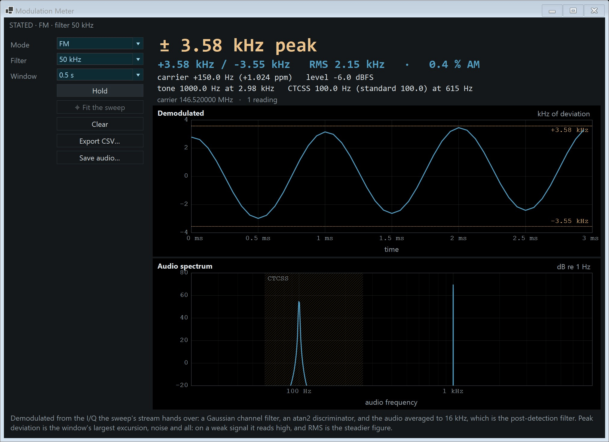
Modulation meter: a stated FM test signal: deviation each way and RMS, the 1 kHz tone and a 100 Hz CTCSS tone.

Phase noise: off a reference recording: the curve, the analyser’s own limit, the stretch the resolution filter hides shaded, and a reference curve.

Two-tone test: a reference recording’s tones and products against PEP, the worst product against your limit, and the products against time.
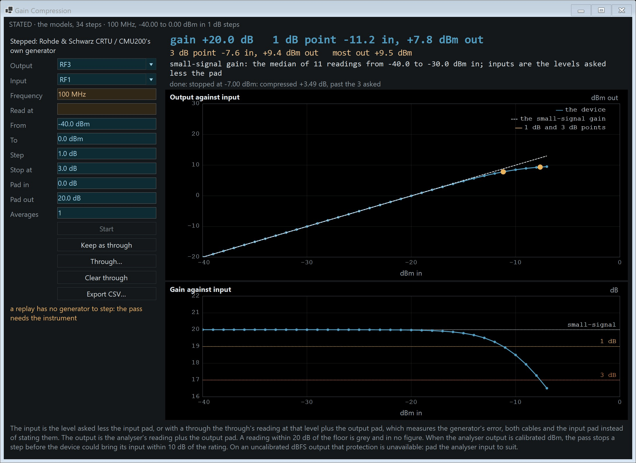
Gain compression: on the instrument models, the CMU’s generator into a model amplifier: output and gain against input, and the 1 dB and 3 dB points.

Transmitter measurements, harmonics: a 100 MHz carrier on a reference recording, H2 to H5 in dBm and dBc, and the THD verdict against the limit.

Wideband survey: the FM band surveyed on the CMU’s model, pass after pass, the heat map, the spectrum cell by cell with its maximum, mean and least, and what was keyed for how long.
🎯 A network analyser
What an antenna, a cable or a component sends back, and what a filter lets through, from whatever the bench has.
🔌 Through a bridge, on any bench
A return-loss bridge between any generator and any analyser on the list gives VSWR and return loss, calibrated against an open, a short and a load. Without a phase reference that is a scalar measurement, and the window says so: the bridge’s directivity sets a floor no scalar calibration can remove, and readings near it are marked as bounds rather than measurements.
🎯 Vector, on a NanoVNA or with a splitter
On a NanoVNA, S11 and S21 read raw and corrected by the window’s own open, short, load, through and isolation, with S21 as an enhanced response. Or a splitter at the stimulus and a second receiver input, on a Pluto, a B210 or the oscilloscope, makes any of those benches vector too.
📐 Every way of drawing it
VSWR, return loss, a Smith chart, R + jX, phase, group delay, Q and the time domain with a gate, every quantity at every marker, and a summary in words: the best match, the 2:1 bandwidth, the resonances, and what would match it.
🧰 Kits, fixtures and files
Calibration kits by their standards’ models, a fixture or a cable taken off the readings from its Touchstone file, calibrations saved and reapplied, and Touchstone out. An SWR meter reads one frequency continuously against time, for tuning an antenna.

Smith chart: a 20 m dipole from a reference file, impedance at two markers, and the summary of where it matches and how to match it.

On a NanoVNA: the NanoVNA’s model with a 20 m band-pass filter between its ports: the filter’s transmission, return loss and group delay, calibrated with open, short, load, through and isolation.
📻 Transmitters and receivers on the bench
One instrument keyed into another through a cable, and measured against a list of checks.
📤 Transmitter test
The source keys itself into the analyser: each carrier’s level and counted frequency against what was asked, the lines beside it, its harmonics, spurs across the analyser’s whole range, its linearity, its output across a band, how fast it settles, a pulse against its duty, and how fast it hears again after it stops.
Before anything is keyed, the loudest level asked is held to the input’s ratings and the pad’s watts. Run on a HackRF, two B210s, a Pluto, a Hermes Lite 2 and a NanoVNA, keyed into a CMU 300.
📥 Receiver sensitivity
A receiver’s 12 dB SINAD, its minimum discernible signal, or the level its squelch opens at: the CMU’s generator into the antenna socket and the receiver’s audio into the CMU-B41, or into the PC from a transceiver’s own USB sound card.
Every pass runs a control first, the cable off, so a reading that was leakage is withheld rather than reported. A receiver with a CAT port is set up and tuned by the pass itself.
🎙️ The audio option
The CMU-B41 fitted inside the CMU: a tone out, and a voltmeter, counter and distortion meter in, with SINAD and THD+N. It is found by asking the instrument, because the instrument’s own option list does not mention it.
📋 Transceiver suite
A ham transceiver tested by a plan: its power against what was asked, its harmonics and spurs against a cited rule, its receiver’s SINAD, MDS and squelch, a carrier at a time and rested by the plan’s duty. Each result is kept as it finishes, so a plan that stops carries on where it stopped, and the lot becomes a test report.

Transmitter test: on the instrument models, a HackRF keyed into the CMU at four carriers from 100 MHz to 2 GHz, its harmonics, spurs, settle and turnaround, and every held check passed.

Receiver sensitivity: on the CMU’s model and its test receiver, 12 dB SINAD on three 2 m channels, the curve against the generator’s level, and the control that proves the reading is the receiver’s.

Transceiver suite: on the instrument models, a plan of power, harmonics and SINAD, run a unit at a time, each result kept as it finishes.

The audio option: on the CMU’s model, the CMU-B41’s tone looped from AF OUT to AF IN, its level in mV and dBu, SINAD and THD+N.
🎯 Level calibration
An SDR reads digital full scale. This makes it read dBm, and says every time which of the two you are looking at.
Every frame says what its levels are measured against, and every caption follows it: dBm from the instrument’s own calibration or a stored table, dBm (fs) from a full scale you stated, dBFS, or dB rel under an AGC. Only dBm has a figure in watts, and a level in dBFS is never drawn against a rating in dBm.
The calibration window takes a table of corrections over frequency, by substitution: the bench’s generator into the receiver, then the same cable end into a receiver you trust, such as the CMU’s own input. The trusted receiver can be a third box; with none, a source with a stated accuracy, or a power meter whose readings you type, makes a lower tier, and the table says which. Tables are kept per unit and per state, with the gain law and the IF response beside them, and a transmitter gets a table of its own. Tables have been taken on three RTL-SDR dongles, a HackRF, a B210 and a Hermes Lite 2, and the dongles’, the HackRF’s and the Hermes Lite 2’s verified to within 0.6 dB of the reference.

A level table: an RTL-SDR Blog V4’s table from 23 MHz to 1.77 GHz against the CMU’s input, with its drift and linearity, shown in a stated state.

The generator, stepping: a carrier stepped across 88 to 108 MHz, the picture drawn as the analyser would see it, and the steps against time.
🎨 Ways of looking at it
The trace never goes away. Everything here changes the pane under it, or draws on top of it.
🌌 Four ways to see history
A ring waterfall with a cursor line, a continuous scroll, a 3-D terrain on the GPU, or a split with the terrain above and the scroll below joined at a seam that is the same instant in both. Fourteen colour palettes, chosen by looking at them.
✨ Phosphor persistence
Five pictures of where the trace has been, a density count among them, and a decaying peak envelope beside them. It is deliberately not called peak hold, because the trace table already has a max hold that holds for ever.
🔍 Zoom, a lens and a navigator
Wheel to zoom about the pointer, drag to select a band, drag the scale to pan; at full span the drag retunes the instrument. A zoom lens opens a second view in a window of its own, with its own waterfall, and a navigator strip shows the whole sweep downsampled by maximum, so it cannot lose a narrow carrier.
🌌 A 3-D spectrogram you can click on
A block of recorded sweeps in its own window that you can orbit all the way round and pick a point on: it reads back the frequency, the time and the level, and draws the spectrum at that instant and the history at that frequency on the surface.
Split view: terrain over scroll, the two halves meeting at the same instant with history running away in both directions.

Phosphor, spread mode: the persistence cloud over the trace shows how much room each modulated signal on the demo band actually occupies.
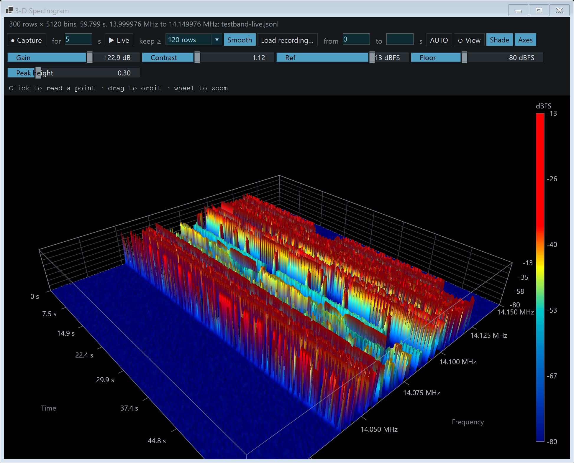
3-D spectrogram: its own window, orbited off the default angle, with the time and frequency axes and the colour bar showing.

Peak annotations: the plot labelling the strongest signals on the band without a marker being placed.
The palette menu, open
The fourteen tiles, each a synthetic waterfall frame through that palette. This one has to be a screen capture, because a drop-down is not in a rendered window shot.
Open View → Waterfall → Palette and capture the drop-down.

The same band in three palettes: Viridis, Inferno and Classic (green), left to right. The ramp changes what you notice.
⚠️ Leaving it running
The parts that are meant to be used with nobody in the room.
Arm a mask
Every sweep is checked against an upper and lower limit in hertz and dBm. One entry per trigger, not one per violating point per sweep, then a hold-off and a re-arm on a clean sweep.
Or set a rule
Any live measurement, a comparison, a threshold, and a dwell in sweeps. It rearms on hysteresis, so a reading sitting on its threshold does not write a row every other sweep.
Keep what caused it
Twenty sweeps before and sixty after, written to a recording named for the local time so it matches the log row. A second alarm extends the window rather than opening another file.
🔒 Nothing an alarm does can open a dialog
An alarm fires at 03:41 with nobody in the room. A file-save prompt waiting for a click has recorded nothing and stopped the watch as well, so the recorder names its own file and the script action is compiled and trusted when you tick the box, never at the moment it fires.

Trigger log: mask violations as rows, severity in the row colour, and the summary line underneath.

A limit mask, armed: a spurious and harmonic mask over the transmitter recording, with the trigger panel reporting what it caught.
📄 Reports
Every result kept, and documents made from them with your name on the letterhead.
📚 The results library
Every measurement collected into a test report is kept, and so is every unit of a transceiver suite and every command-line measurement you ask to keep: its figures, its verdict and the sentence beside it, its picture and its data, and where it was taken: the device, the operator, the instrument, the generator and the path.
📑 Documents, in HTML or PDF
Tick the results and choose a full report, a summary or a data sheet, numbered and addressed. The letterhead, logo and signature come from the Identity page in Setup. The test report window collects every open measurement window as it stands into one file.

The results library: three kept results, two of them ticked into a numbered report for a radio club, with the preview of what will be written.
✅ What is checked, and what is not
Written down here for the same reason it is written on the screen: an analyser that quietly reports a plausible wrong answer is worse than one that says it cannot tell.
The expected answers in the self-test were produced by a separate implementation in another language, and that separation is the whole guarantee: a test that computes what it expects using the code under test proves only that the code is deterministic. Every instrument then has a bench of its own that drives the real acquisition path against the real unit, reads its state first and puts it back afterwards: 129 checks on a CMU 300, 82 on a HackRF, 80 on an OWON generator, 76 on an SDRplay.
🔧 What running it against a real instrument found
The software model of the CMU200, written from the command reference, was wrong in several places the manual had led it to. Frequencies are hertz, not kilohertz, so connecting to an instrument on the FM band reported 88 to 108 gigahertz. The resolution bandwidth is clamped silently, and the floor it clamps to rises with the span. Errors are queued rather than reported, so a rejected setting looked exactly like an accepted one. And the reference level, which the data sheet says slides the whole measurement window, does not move the noise floor on this instrument at all.
The other instruments were no different. The CMU200 emits on all three connectors with its generator switched off. A HackRF went silent after a retune out of one band unless the tune was sent twice. A Hermes Lite 2 receives on its transmit oscillator unless one bit is set, and saturates near 2 W rather than 5. Each is handled, and each is in the handbook.
⛔ What has not met hardware yet
The receiver tests and the transceiver suite. They have run on the instrument models and on Hamlib’s dummy rig; no real receiver’s sensitivity has been measured and no real transceiver has been keyed by the suite.
The vector routes by a reference input (a splitter and a second receiver on a Pluto, a B210 or the oscilloscope) have run on the models only. The bridge route has met the CMU 300 from the command line, and the NanoVNA its own unit; the window’s keys and the SWR meter have not met hardware.
The relay has been run on one PC through its own loopback, not yet between two machines.
🎬 It works with no instrument
Which is how you can try it before you buy anything, and how every picture on this page was taken: on the demo band, a reference recording or the instrument models.
With no instrument to reach, START runs a live test band: a 480 ksample/s receiver centred on 14.080 MHz, synthesising twenty-three signals across the 20 m amateur band at their real frequencies and relative levels. CW, PSK31, RTTY, Olivia, Contestia, FT8, FT4, SSB voice, FreeDV, SSTV, WEFAX, APRS and NAVTEX.
These are I/Q samples, not a saved picture. FT8 keys up on its 15 second cycle, CW is keyed, speech moves the SSB signals, APRS sends a packet every twenty seconds, and everything fades at its own rate. A zoom takes a longer FFT and shows detail that was not there before, the VFO’s Listen row plays the SSB voice through your speakers, and the modulation meter and the I/Q recorder read the same stream the spectrum is drawn from. One carrier is a beacon and never moves, so there is something steady to watch the rest against.
Or choose the model analyser: a simulated instrument behind the real acquisition path, so every control can be tried, and every measurement window run, with no hardware at all.
👁️ It never stops saying what it is
The window caption and the status line read DEMO for as long as it runs, so a screenshot taken in demo mode cannot be passed off as one taken from an instrument. And demo mode is never entered by accident when an instrument can be reached: one that is merely switched off reports its own error rather than silently becoming a test band.
Demo mode running, caption visible
A capture that includes the title bar and the status line, so the DEMO label is in the picture. This one needs a real screen grab rather than a rendered shot, because the title bar is drawn by Windows.
Launch with no VISA runtime, press START, and capture the whole window
including the title bar.
🖥️ What you need
Instrument
- ● Any one of the fourteen above, or none, for the demo and the model
- ● A CMU200 needs the RF non-signalling function group; its generator and the CMU-B41 are optional
- ● Optional: a second instrument as the source, a relay board, a transceiver
Connection
- ● GPIB and USB test instruments: a 64-bit VISA runtime (NI-VISA, Keysight IO Libraries or R&S VISA)
- ● SDRs: the maker’s driver or library, which Device Setup checks, and for some fetches from the publisher when you ask
- ● No vendor runtime is bundled: each is the one you install
PC
- ● Windows 10 or 11, x64
- ● A wide monitor helps. The layout works from 1280 px up
- ● Optional: any GPU, for the accelerated terrain
- ● Optional: CPython with numpy, for Python scripts
- ● Optional: a USB volume knob, as a VFO
🧰 Help → Device Setup
One card per kind of instrument says what is installed, what Windows sees and with which driver, and what works right now, and gives the steps that fix what does not. Where a step is a download, nothing is fetched until you press the button, after a box that names the file, the publisher, the licence and where it goes, and only the exact file expected is kept. Checking opens no instrument.
🔒 x64, and why
No ARM64 VISA runtime exists, so this is an x64 application. It uses whichever VISA runtime you have registered, and looks for it in the registry rather than by trying and catching, so running without one is a decision it makes cleanly and tells you about.
▶️ Getting a trace on screen
Check the PC
Help, then Device Setup. A card that says Ready is ready; any other says what it is waiting for and offers the next step.
Press DETECT
On the Connection page in Setup. It walks the GPIB bus, the USB devices and the network, and fills in the instrument list, keeping every unit it finds rather than only the first. Choose the one to use and press Set active.
Press START
Connecting adopts the instrument rather than overruling it. Whatever it can report (the frequencies, the bandwidth, the reference level, the connector) is read back and shown, and a command goes out only when you change one.
Pick a band
The preset recall on the Frequency panel, or the amateur band plan beside it, or a click on the plot to move the VFO.
Watch the bandwidth, and the units
An instrument may take a wider resolution bandwidth than you asked for, and the Capture page shows what it actually took. An SDR’s levels are dBFS until it is calibrated, and every caption says so; the calibration strip offers to take a table when one would help.
📁 Everything it writes is plain text
Readable, diffable and editable by hand, apart from the pictures, the videos and the raw I/Q. Nothing is in a database and nothing is in a proprietary container.
| File | Holds |
|---|---|
.jsonl | A sweep recording: a header saying which instrument and which frequency axis, then one line per sweep, so a recording survives a crash with only its last line missing. |
.sigmf-meta, .sigmf-data | An I/Q recording, in the open SigMF format other SDR software reads. |
.ovl | An overlay or a trace snapshot, with the band it covers. |
.msk | A limit mask. Absolute in hertz and dBm, or relative in dBc with the anchor rule stated. |
.cal, .lvl, .ncal, .kit | A response calibration, a level table, a network calibration and a calibration kit, each saying what it was taken against and when. |
.s1p, .s2p | Touchstone: a reflection out, a fixture in. |
.csv | Exported traces, logs and every measurement window’s data. A survey writes rtl_power’s own CSV. |
.json | A kept result, its picture and data beside it, for the reports. |
.html, .pdf | A test report or a document merged from the results library. |
.csx, .py | A script, in C# or Python. |
.mp4 | A window recording. H.264, no sound. |
settings.json | Everything configurable, in one file under your local app data, not in the registry. |
🔧 It automates
Most measurements have a command-line mode that runs them with no window: the bench of checks, a level calibration, a transmitter or receiver test, a survey, the network analyser, phase noise, the modulation meter, a transceiver suite and a report composed from the results. Raw SCPI with timing, a mirror of every byte on the bus, and the display rendered to PNG at any size, theme, view and panel. Every picture on this page was rendered that way, by the application itself.
📖 The handbook
Fifty-three chapters, control by control.
The application ships with a full operator’s handbook, reachable from Help inside the application. It documents every instrument and what it can and cannot do, every control and window, what goes down the bus and when, every file format, every command-line switch, the keyboard and mouse reference, and a troubleshooting chapter for the failures that are the instrument’s rather than the software’s.
It also carries the caveats: which numbers have been measured against a real instrument, which have only been checked against a model of it, and which have never been checked against hardware at all.
The handbook open in a browser
Shows that the documentation is real and substantial. Capture the contents rail and a section with a table in it.
Open docs/help.html in a browser and capture it.
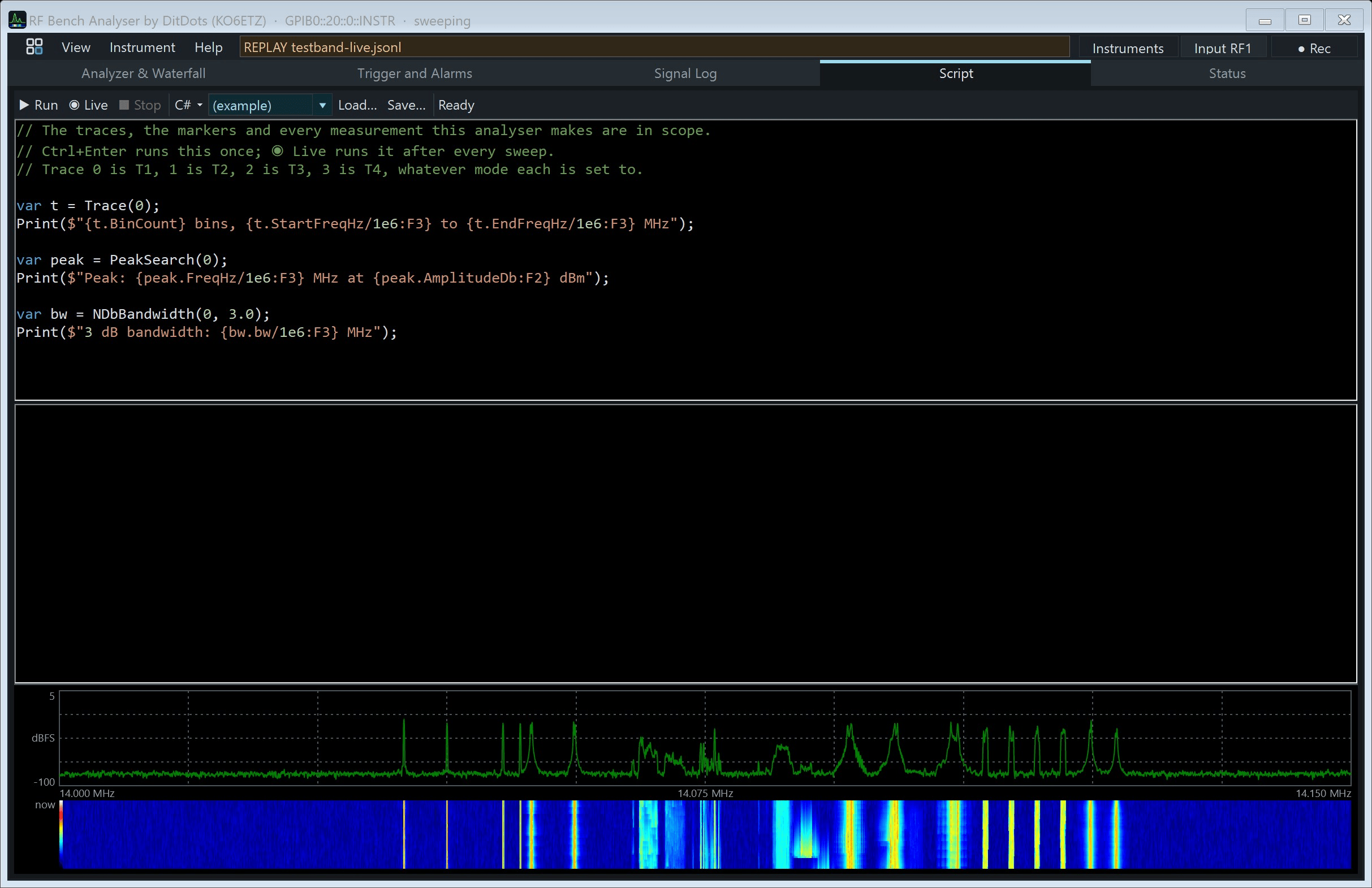
Scripting page: a script that reads the traces and measures the peak and the 3 dB bandwidth of this sweep.
📡 RF Bench Analyser
Built by an amateur who wanted a proper front panel on a very good instrument, and then on every other box on the bench. If you own a CMU200 that has been sitting under the bench because nobody can face the menu tree, or a drawer of SDRs that have never read a level you trust, this is what they were waiting for.
$9.99 when it lands. One purchase, no subscription, no licence server, no account. Windows 10 or 11, x64.
Click anywhere or press Esc to close