Interactive Voronoi & power diagrams — for points and line segments, in 2D and 3D.
Draw wells, roads, towers or components and watch their territories re-tessellate in real time — or switch to 3D and slice, explode, animate and measure polyhedral cells in a box, a sphere, a gem, a vase or a chess pawn. Weighted cells, grouped networks, CVT optimization and exact area and volume analytics — running entirely in your browser.
▶ Launch the app Open in 3D ▶ Watch the walkthrough Read the manualSee it in three minutes
Clicking points and dragging segments into new cells, weights and polylines, then 3D: section planes, exploded views, eleven shapes and live animations.
 3:17
Short on time? Watch the 0:58 highlights on YouTube.

New in 2.0: 3D cells
Everything Voronoi DD does in the plane now works in space. Points and 3D segments (wells, vessels, fibers, cables) partition a box, a sphere, a capsule, a gem, a vase, a bone or a chess pawn into exact polyhedral cells — weighted, grouped, sliced, exploded, animated and measured. Flip the 2D | 3D switch at the top of the app’s sidebar.


Slice it
Cut the tessellation with a plane on X, Y, Z or any custom normal: clip either side, keep a slab, or show the section only. Every polyhedron is clipped exactly and the cut faces are drawn in the cell’s color, while a linked 2D panel shows the cross-section map with its total area.
Ctrl+click on the plane adds a new seed right there — its cell appears in 3D on the next recompute. Sweep animates the plane through the domain.


Take it apart
Explode cells away from the center (radially or along one axis), shrink them about their centroids, peel the outer layers like an onion, hide edge cells, keep only a metric range or one group, or isolate a cell with its neighbors. Hidden cells stay as faint glass for context.
Peel two layers off a BCC iron crystal and the interior is a perfect stack of 14-faced truncated octahedra — exactly what crystallography predicts.

Measure it
Per cell: volume, surface area, faces, neighbors and the contact area of every wall, sphericity, elongation (from the inertia tensor), equivalent diameter and depth layer. Color by any of them, hover for an info card, and export the whole table — plus the weighted contact graph — as CSV.
Domain volumes are exact and the cells tile them exactly, so the numbers are usable as declustering weights, drainage volumes, free volume or local fiber fraction.


See it your way, take it with you
Solid, solid + edges, glass (seeds and inner walls show through) or wireframe; perspective or orthographic; camera presets, auto-rotate and vertical exaggeration for geoscience models.
Export OBJ (Blender, MeshLab, CAD), VTK (ParaView) and a printable strut-lattice STL — the classic Voronoi foam for 3D-printed scaffolds and infill.


Any shape, not just a box
Fill a box, sphere/ellipsoid, cylinder, capsule, cone, egg, brilliant-cut gem or hexagonal prism — or the non-convex vase, bone and chess pawn. Every shape is inscribed in the X/Y/Z bounds, so the bounds set its size and proportions.
The non-convex shapes are split into exact convex slabs behind the scenes; the seams are invisible and volumes still add up to the shape’s volume exactly. Wireframe + strut-lattice STL turns the vase or the pawn into a printable Voronoi lattice.
 1:27
Animate it
Nine presets: turntable, explode / implode, slice sweep, onion peel, print build-up (cells appear layer by layer like a 3D printer), grow from center, live Brownian motion and weight pulse that re-tessellate every frame, and CVT relaxation.
Record any of them: WebM in the browser, GIF or MP4 in the desktop app. The video plays them on twelve of the 3D datasets in eight domain shapes, rendered by the app itself.
Sixteen 3D datasets
Radical Voronoi of iron atoms: truncated octahedra, a vacancy, a chromium substitution and a carbon interstitial.
Laguerre grains from lognormal grain sizes — face statistics close to Kelvin’s foam limit.
Tumor cells in an ellipsoid and three grouped capillaries: each vessel’s oxygen-supply volume.
Vertical, deviated and horizontal wells in a stacked reservoir; injectors weighted for pressure support.
Composited samples along inclined holes: each cell is a sample’s volume of influence.
Four floors of access points and a leaky-feeder shaft — slice each floor to read its coverage.
Clusters, filaments and voids: density = 1 / cell volume; the biggest cells are the voids.
Radical weights per species give each particle its share of space — local free volume.
A dense cortical shell around an open core, in a cylinder — export it as a printable lattice.
Fibers as 3D segments plus filler particles: the matrix region each fiber reinforces.
A relaxed lattice filling a vase — the classic printed Voronoi vase, ready for STL export.
Cells that follow the turned profile of base, stem, collar and head.
A brilliant-cut stone split into faceted shards — explode it.
The 24-cell stage with lineage names (ABalaa…, MSa, Ea, P4) inside its eggshell.
Dense trabecular ends and long shaft cells in a bone-shaped domain.
Laguerre-packed pellets in a size-0 capsule; void space per pellet.
What it does
A Voronoi diagram assigns every location to its nearest seed. Voronoi DD extends the classic picture three ways that real problems need: segments as first-class seeds, weights that grow or shrink territories, and groups that make a network act as one unit.

Weighted cells (power diagrams)
Give an element a weight and its territory grows — a macro tower out-reaches a small cell, an anchor store out-pulls a kiosk, a big grain swallows its neighbors. Mathematically a power / Laguerre diagram: walls stay straight, they just shift toward the lighter site.
Editing is live: hold Shift and scroll the mouse wheel over any element and watch its cell inflate or deflate.
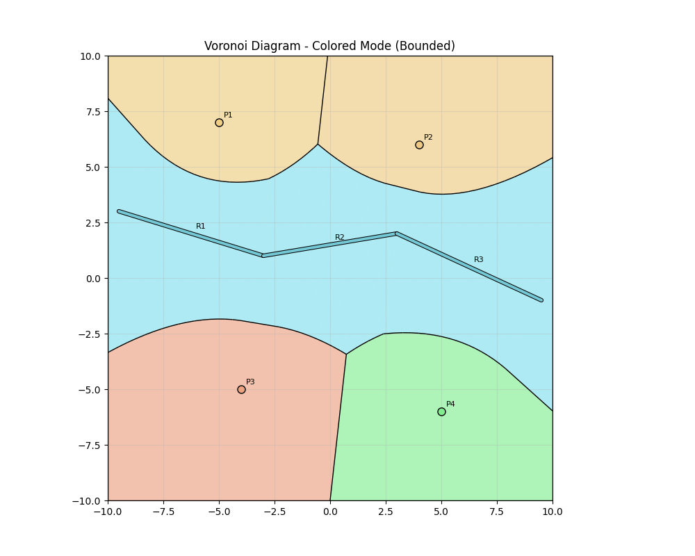
Groups: networks act as one
A river drawn as three chained segments shouldn’t have internal walls at the joints. Elements sharing a group name get one color, merged cells and aggregated analytics — one riparian corridor, one metro catchment, one power rail.
Turn on Auto-group chained segments and any polyline you draw is detected and grouped automatically.
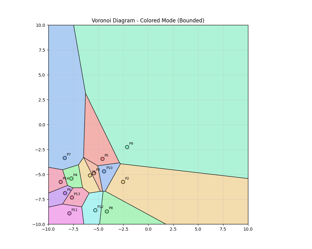

Optimize with Lloyd / CVT
“Spread these facilities evenly over the territory” is a solved problem: Lloyd’s algorithm moves every point to its cell’s centroid and repeats. Watch 14 clustered points relax into a uniform centroidal Voronoi tessellation — while segments stay fixed as infrastructure the points arrange themselves around.
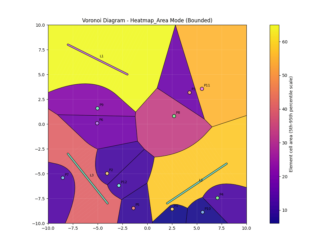
Analytics, not just pictures
Five visualization modes including a distance heat map (true point-to-segment distance field) and a cell-area map that instantly shows over- and under-served territory.
Hover any cell for its exact area, weight, group and the list of neighbors it shares a wall with. Export areas writes a CSV with exact clipped areas plus the full neighbor graph — the input for allocation and weighting workflows.
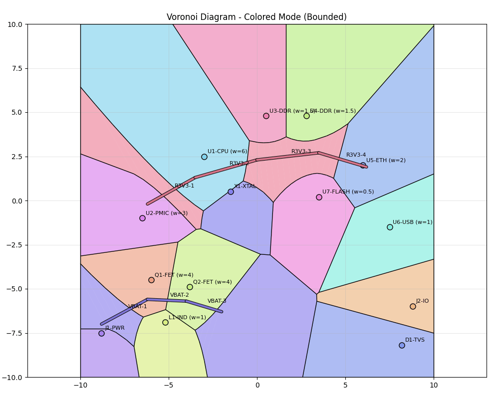
Edit everything in real time
Click to add a point. Drag to add a segment. Ctrl+drag to move an element and watch the whole map re-tessellate live under your cursor. Right-click deletes, Ctrl+Z undoes fifty steps back.
Every regeneration runs the full scientific-Python geometry engine (numpy + scipy, compiled to WebAssembly) in 10–60 ms — locally, in your browser tab.
Eleven industry datasets built in
Each sample pairs points with segments the way that domain actually uses proximity partitions, with real-world element IDs and a “things to try” guide shown in the app.
Vertical wells vs horizontal laterals; cell area ≈ drained acreage. Stimulated wells carry weights.
Components weighted by dissipated power; grouped power rails. First-order copper-allocation map.
Schools weighted by capacity, grouped avenues capturing frontage corridors.
Stores (weighted anchors) vs arterial roads modeling drive-by capture.
Macro vs small cells as a power diagram; a grouped highway corridor.
Capacity-weighted substations and grouped transmission lines.
First-due districts per fire station; a grouped river shows barrier distortion.
A grouped canal network (main + branches) vs wells — segments at their best.
Lognormal grain-size weights make a true Laguerre diagram; dislocation lines cut defect zones.
Two grouped metro lines vs surface stops: walk-to-line vs walk-to-stop planning.
Cell area per borehole = its polygonal declustering weight; grouped fault traces partition blocks.
User manual
Getting started
- Open the app — the first visit downloads the Python/scipy runtime (~30 MB, cached afterwards; later visits start in seconds).
- Pick a sample dataset — its description and “things to try” appear in the sidebar — or start from the blank canvas.
- Click and drag on the map. Everything regenerates as you edit.
Mouse & keyboard
| Input | Action |
|---|---|
| left click | add a point (auto-ID P1, P2, …) |
| left drag | add a segment with a rubber-band preview (L1, …) |
| Ctrl + drag | move the nearest point or segment endpoint — the diagram re-tessellates live |
| right-click | delete the nearest element |
| Shift + wheel | adjust the nearest element’s weight (live power diagram) |
| wheel | zoom at the cursor |
| middle-drag | pan the view |
| hover | highlight the cell + info card: area, weight, group, neighbors |
| Ctrl+Z / Esc | undo (50 steps) / cancel an in-progress drag or move |
Visualization modes
| Basic diagram | cell walls only, in blue |
| Colored cells | one pastel per element or group + black walls — the workhorse view |
| Boundaries only | thin black walls, no fills |
| Heat map (distance) | distance-to-nearest-element field (segments use true point-to-segment distance) with a colorbar |
| Heat map (cell area) | cells colored by their element’s total area, 5–95th percentile scale, with a colorbar |
Boundary modes & bounds
Bounded clips the diagram to the X/Y bounds — areas are exact and physically meaningful. The clip box expands automatically to the window’s shape so cells always fill the canvas, and it re-clips when you resize. Infinite look lets cells run past the viewport for the classic unbounded picture (areas are then only relative).
Weights, groups and Lloyd
Weights are in squared-distance units: positive grows a cell, negative shrinks it, and a massively out-weighted element can end up with no territory at all (it is “hidden”). A segment’s weight applies to its whole corridor. Groups come from the dataset’s Group column or the auto-group toggle. Lloyd step / Relax (CVT) move every point to its cell centroid (segments never move) — Bounded mode only.
Data in & out
ID,X,Y,X2,Y2,Type,Weight,Group
V-01,-7.35,6.53,,,point,2.5,
H-01,-8.5,-1.5,-2.5,-0.3,line_segment,,
R1,-9.5,3.0,-3.0,1.0,line_segment,,River
Import CSV / Export CSV use this format — Weight and Group are optional, and files are fully interchangeable with the desktop app. Export areas writes one row per element with its exact clipped cell area and a semicolon-separated Neighbors list (which elements share a wall) — the analysis product behind every allocation workflow.
3D mode
Switch with the 2D | 3D toggle (or open ditdots.com/voronoi/#3d). The 3D view needs WebGL, which every current desktop browser has.
| Input (3D) | Action |
|---|---|
| left drag / right drag / wheel | orbit / pan / zoom |
| hover / click | info card (volume, surface, faces, neighbors, sphericity, …) / select the cell |
| Ctrl + click | add a point on the active section plane — a new cell appears |
| right-click | delete the element under the cursor |
| Shift + wheel | change the weight of the cell under the cursor |
| Ctrl+Z / Esc | undo / clear the selection |
Domain: box, ellipsoid, cylinder, capsule, cone, egg, gem, hexagonal prism, vase, bone or chess pawn, inscribed in the X/Y/Z bounds. Animate: preset, duration, loop, play/stop and Record WebM. View: style, color-by metric with colorbar, colormap, vertical exaggeration, field of view, perspective/orthographic, camera presets. Slice: plane axis or custom normal, position, clip below / above / slab / section-only, cut caps and the 2D inset. Decompose: explode (radial or per axis), shrink, peel layers, range and group filters, isolate. Generate: uniform, Poisson-disk, clustered, SC/BCC/FCC/HCP lattices, graded, radial, random fibers — then Lloyd / CVT in 3D.
ID,X,Y,Z,X2,Y2,Z2,Type,Weight,Group
Fe-012,2.15,2.15,6.449,,,,point,1.5876,
V-01,300,300,-2105,300,300,-2395,line_segment,,
3D files add a Z column (importing one in 2D mode switches to 3D automatically). Exports: dataset CSV, cell metrics CSV, contact graph CSV, section CSV, OBJ, VTK, strut-lattice STL and a PNG of the view.
Tips & troubleshooting
| First load is slow | The Python runtime (~30 MB) downloads once from a CDN and is cached; later visits start in seconds. |
| A weighted element has no cell | It is out-weighted (“hidden”). Lower the neighbors’ weights or raise its own with Shift+wheel near its marker. |
| Walls between the reaches of a polyline | Intentional until grouped — enable Auto-group chained segments or set a Group in the CSV. |
| Lloyd button does nothing | It needs Bounded mode and at least one point element; segments alone can’t relax. |
| Areas look enormous | You are in Infinite look; switch to Bounded for physically meaningful areas. |
| Exact parabolic arcs? | The browser uses the fast sampled solver. The desktop app adds an exact segment-Voronoi solver (Boost.Polygon) with true parabolic bisectors. |
| 3D view stays blank | WebGL is disabled or blocked (some remote-desktop sessions and locked-down browsers). Enable hardware acceleration and reload. |
| 3D segment cells look faceted | Segments are sampled into sub-seeds, so the curved surfaces around them are slightly scalloped. Cell volumes are still exact for the sampled geometry. |

Map your territory — or your volume
▶ Launch Voronoi DD Open in 3DPart of Dit Dots by KO6ETZ — ham radio · electronics · software.
Geometry: numpy + scipy running in-browser via Pyodide; 3D view: three.js.