Interactive Voronoi & power diagrams — for points and line segments.
Draw wells, roads, towers or components and watch their territories re-tessellate in real time. Weighted cells, grouped networks, CVT optimization and exact area analytics — running entirely in your browser.
▶ Launch the app Read the manual
What it does
A Voronoi diagram assigns every location to its nearest seed. Voronoi DD extends the classic picture three ways that real problems need: segments as first-class seeds, weights that grow or shrink territories, and groups that make a network act as one unit.

Weighted cells (power diagrams)
Give an element a weight and its territory grows — a macro tower out-reaches a small cell, an anchor store out-pulls a kiosk, a big grain swallows its neighbors. Mathematically a power / Laguerre diagram: walls stay straight, they just shift toward the lighter site.
Editing is live: hold Shift and scroll the mouse wheel over any element and watch its cell inflate or deflate.
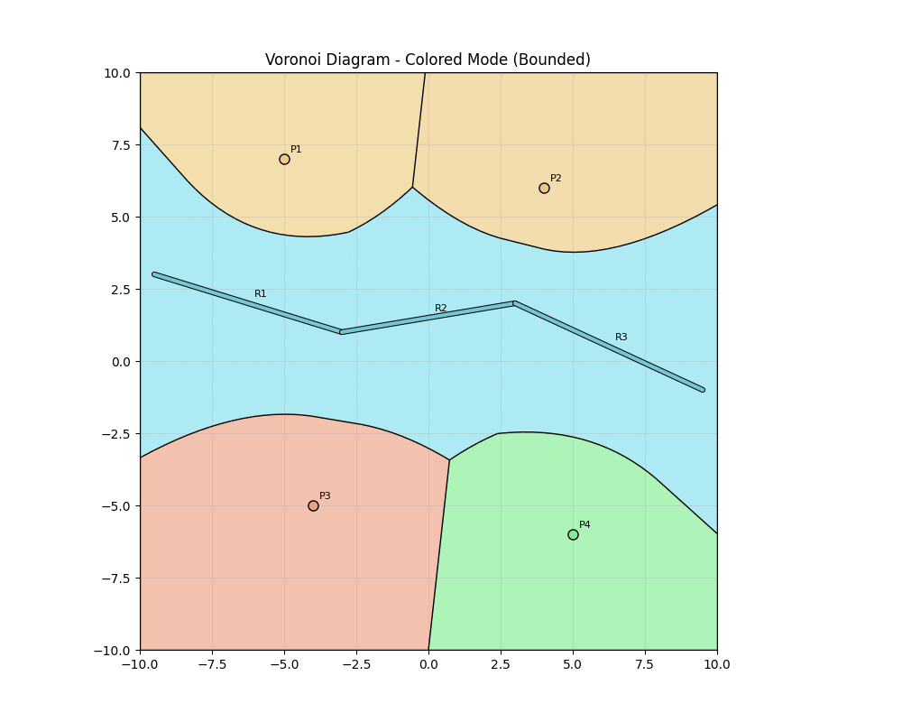
Groups: networks act as one
A river drawn as three chained segments shouldn’t have internal walls at the joints. Elements sharing a group name get one color, merged cells and aggregated analytics — one riparian corridor, one metro catchment, one power rail.
Turn on Auto-group chained segments and any polyline you draw is detected and grouped automatically.
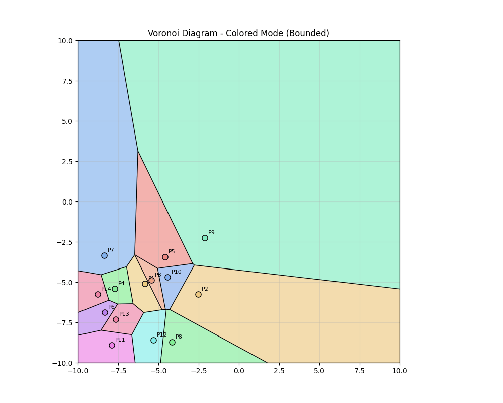

Optimize with Lloyd / CVT
“Spread these facilities evenly over the territory” is a solved problem: Lloyd’s algorithm moves every point to its cell’s centroid and repeats. Watch 14 clustered points relax into a uniform centroidal Voronoi tessellation — while segments stay fixed as infrastructure the points arrange themselves around.
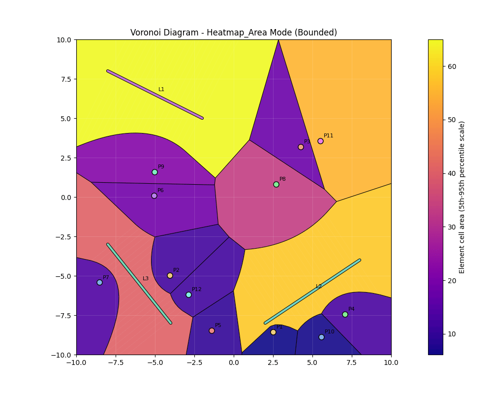
Analytics, not just pictures
Five visualization modes including a distance heat map (true point-to-segment distance field) and a cell-area map that instantly shows over- and under-served territory.
Hover any cell for its exact area, weight, group and the list of neighbors it shares a wall with. Export areas writes a CSV with exact clipped areas plus the full neighbor graph — the input for allocation and weighting workflows.
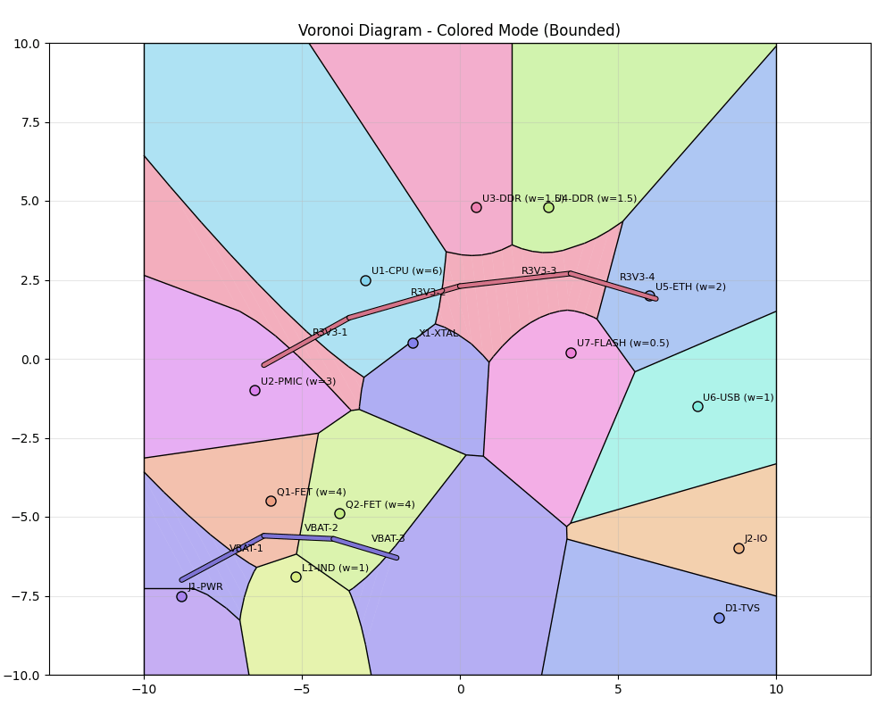
Edit everything in real time
Click to add a point. Drag to add a segment. Ctrl+drag to move an element and watch the whole map re-tessellate live under your cursor. Right-click deletes, Ctrl+Z undoes fifty steps back.
Every regeneration runs the full scientific-Python geometry engine (numpy + scipy, compiled to WebAssembly) in 10–60 ms — locally, in your browser tab.
Eleven industry datasets built in
Each sample pairs points with segments the way that domain actually uses proximity partitions, with real-world element IDs and a “things to try” guide shown in the app.
Vertical wells vs horizontal laterals; cell area ≈ drained acreage. Stimulated wells carry weights.
Components weighted by dissipated power; grouped power rails. First-order copper-allocation map.
Schools weighted by capacity, grouped avenues capturing frontage corridors.
Stores (weighted anchors) vs arterial roads modeling drive-by capture.
Macro vs small cells as a power diagram; a grouped highway corridor.
Capacity-weighted substations and grouped transmission lines.
First-due districts per fire station; a grouped river shows barrier distortion.
A grouped canal network (main + branches) vs wells — segments at their best.
Lognormal grain-size weights make a true Laguerre diagram; dislocation lines cut defect zones.
Two grouped metro lines vs surface stops: walk-to-line vs walk-to-stop planning.
Cell area per borehole = its polygonal declustering weight; grouped fault traces partition blocks.
User manual
Getting started
- Open the app — the first visit downloads the Python/scipy runtime (~30 MB, cached afterwards; later visits start in seconds).
- Pick a sample dataset — its description and “things to try” appear in the sidebar — or start from the blank canvas.
- Click and drag on the map. Everything regenerates as you edit.
Mouse & keyboard
| Input | Action |
|---|---|
| left click | add a point (auto-ID P1, P2, …) |
| left drag | add a segment with a rubber-band preview (L1, …) |
| Ctrl + drag | move the nearest point or segment endpoint — the diagram re-tessellates live |
| right-click | delete the nearest element |
| Shift + wheel | adjust the nearest element’s weight (live power diagram) |
| wheel | zoom at the cursor |
| middle-drag | pan the view |
| hover | highlight the cell + info card: area, weight, group, neighbors |
| Ctrl+Z / Esc | undo (50 steps) / cancel an in-progress drag or move |
Visualization modes
| Basic diagram | cell walls only, in blue |
| Colored cells | one pastel per element or group + black walls — the workhorse view |
| Boundaries only | thin black walls, no fills |
| Heat map (distance) | distance-to-nearest-element field (segments use true point-to-segment distance) with a colorbar |
| Heat map (cell area) | cells colored by their element’s total area, 5–95th percentile scale, with a colorbar |
Boundary modes & bounds
Bounded clips the diagram to the X/Y bounds — areas are exact and physically meaningful. The clip box expands automatically to the window’s shape so cells always fill the canvas, and it re-clips when you resize. Infinite look lets cells run past the viewport for the classic unbounded picture (areas are then only relative).
Weights, groups and Lloyd
Weights are in squared-distance units: positive grows a cell, negative shrinks it, and a massively out-weighted element can end up with no territory at all (it is “hidden”). A segment’s weight applies to its whole corridor. Groups come from the dataset’s Group column or the auto-group toggle. Lloyd step / Relax (CVT) move every point to its cell centroid (segments never move) — Bounded mode only.
Data in & out
ID,X,Y,X2,Y2,Type,Weight,Group
V-01,-7.35,6.53,,,point,2.5,
H-01,-8.5,-1.5,-2.5,-0.3,line_segment,,
R1,-9.5,3.0,-3.0,1.0,line_segment,,River
Import CSV / Export CSV use this format — Weight and Group are optional, and files are fully interchangeable with the desktop app. Export areas writes one row per element with its exact clipped cell area and a semicolon-separated Neighbors list (which elements share a wall) — the analysis product behind every allocation workflow.
Tips & troubleshooting
| First load is slow | The Python runtime (~30 MB) downloads once from a CDN and is cached; later visits start in seconds. |
| A weighted element has no cell | It is out-weighted (“hidden”). Lower the neighbors’ weights or raise its own with Shift+wheel near its marker. |
| Walls between the reaches of a polyline | Intentional until grouped — enable Auto-group chained segments or set a Group in the CSV. |
| Lloyd button does nothing | It needs Bounded mode and at least one point element; segments alone can’t relax. |
| Areas look enormous | You are in Infinite look; switch to Bounded for physically meaningful areas. |
| Exact parabolic arcs? | The browser uses the fast sampled solver. The desktop app adds an exact segment-Voronoi solver (Boost.Polygon) with true parabolic bisectors. |
Map your territory
▶ Launch Voronoi DDPart of Dit Dots by KO6ETZ — ham radio · electronics · software.
Geometry: numpy + scipy running in-browser via Pyodide.