DIT DOTS KO6ETZ HAM RADIO • ELECTRONICS • SOFTWARE 14.074 MHz TX PWR RX

Portfolio

USC CiSoft & Chevron

17 Years at USC CiSoft · 7 as a Chevron Consultant

For 17 years, through 2026, I managed the software lab at USC’s Center for Interactive Smart Oilfield Technologies (CiSoft), part of the Viterbi School of Engineering, including 7 years as a Chevron consultant. This page collects the software I built and led there: production-optimization solvers, waterflood connectivity analytics, computational-geometry engines, and petrophysical modeling tools, all shipped as tested, versioned software running on real field data.


17 Years
Software Lab Manager
7 Years
Chevron Consultant
USC Viterbi
CiSoft
Through 2026
Tenure

Selected Work

Three flagship systems from the lab, then the rest of the bench. Every image below is a real rendered output from the tool described, not a mockup.

01 · Field-Development Optimization

WellScheduler

Multi-cycle production scheduler · v1.0.6 · Python

Schedules well start/stop cycles across a multi-year horizon to maximize field output under a shared facility capacity limit. Each well is modeled with an exponential decline curve, cycle degradation, shut-in threshold, and recovery period. Three solvers on one problem: greedy heuristic, genetic algorithm, and MILP, cross-validated against each other on every run. On the run shown here the greedy heuristic matched the MILP schedule to within 0.04% of total production while solving about twelve times faster.

3,050 Mbbl · Greedy ≈ MILP, Δ0.04%
0.12s vs 1.40s MILP
56.5% Capacity usage
Python PuLP / CBC Genetic Algorithm Tkinter matplotlib NumPy · pandas
WellScheduler main window: optimization parameters, warm-start re-plan controls, a well-data grid of decline-curve properties, and a results panel comparing total production, capacity usage and runtime for the greedy, genetic and MILP solvers.
Main window: parameters, well data, three-solver results
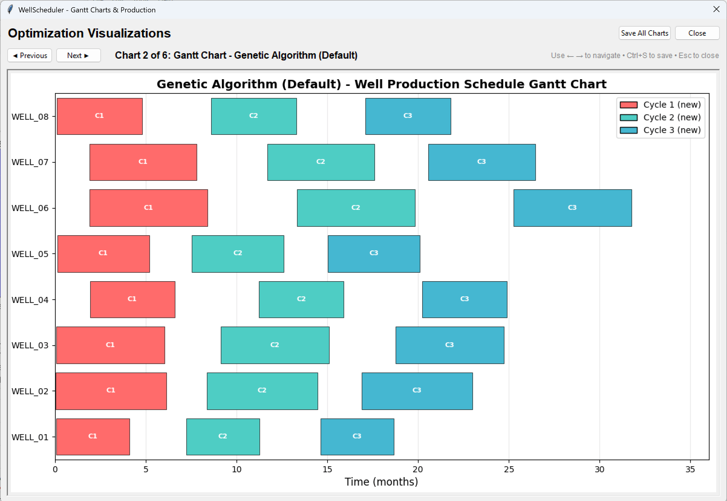
In-app chart viewer showing the genetic algorithm's Gantt chart: eight wells with three colour-coded production cycles each across a 36-month horizon.
Built-in chart viewer: genetic solver schedule, 8 wells × 3 cycles over 36 months
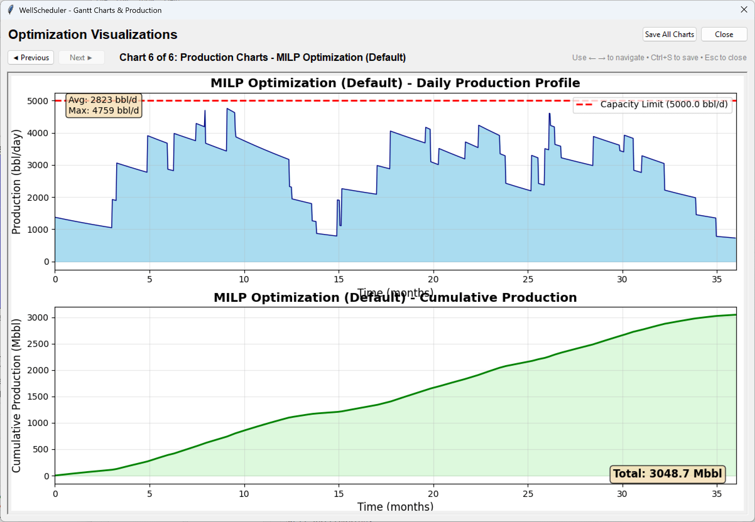
MILP daily production profile tracking beneath the 5,000 bbl per day capacity limit, with the cumulative production curve below it totalling 3,048.7 Mbbl.
MILP: daily profile against the 5,000 bbl/d cap
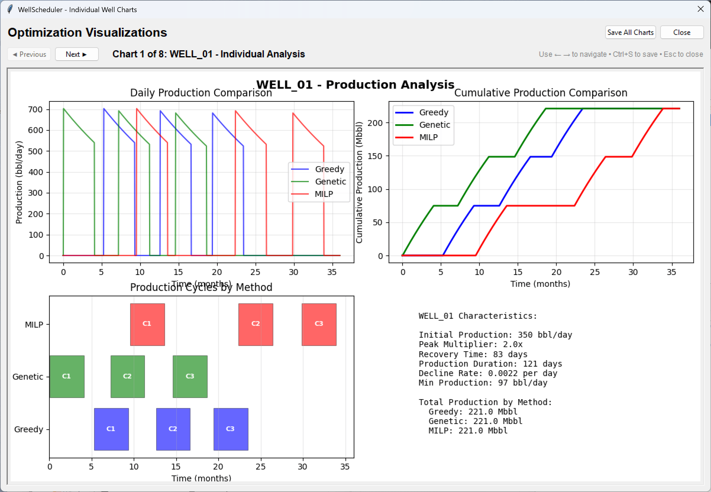
Per-well drill-down for WELL_01: daily and cumulative production compared across all three solvers, the cycle timing each solver chose, and the well's decline-curve characteristics.
Per-well drill-down: all three solvers on one well

Also in this theme: drilling-rig logistics

Rig Routing GA

Weighted multi-depot multiple-TSP · MATLAB

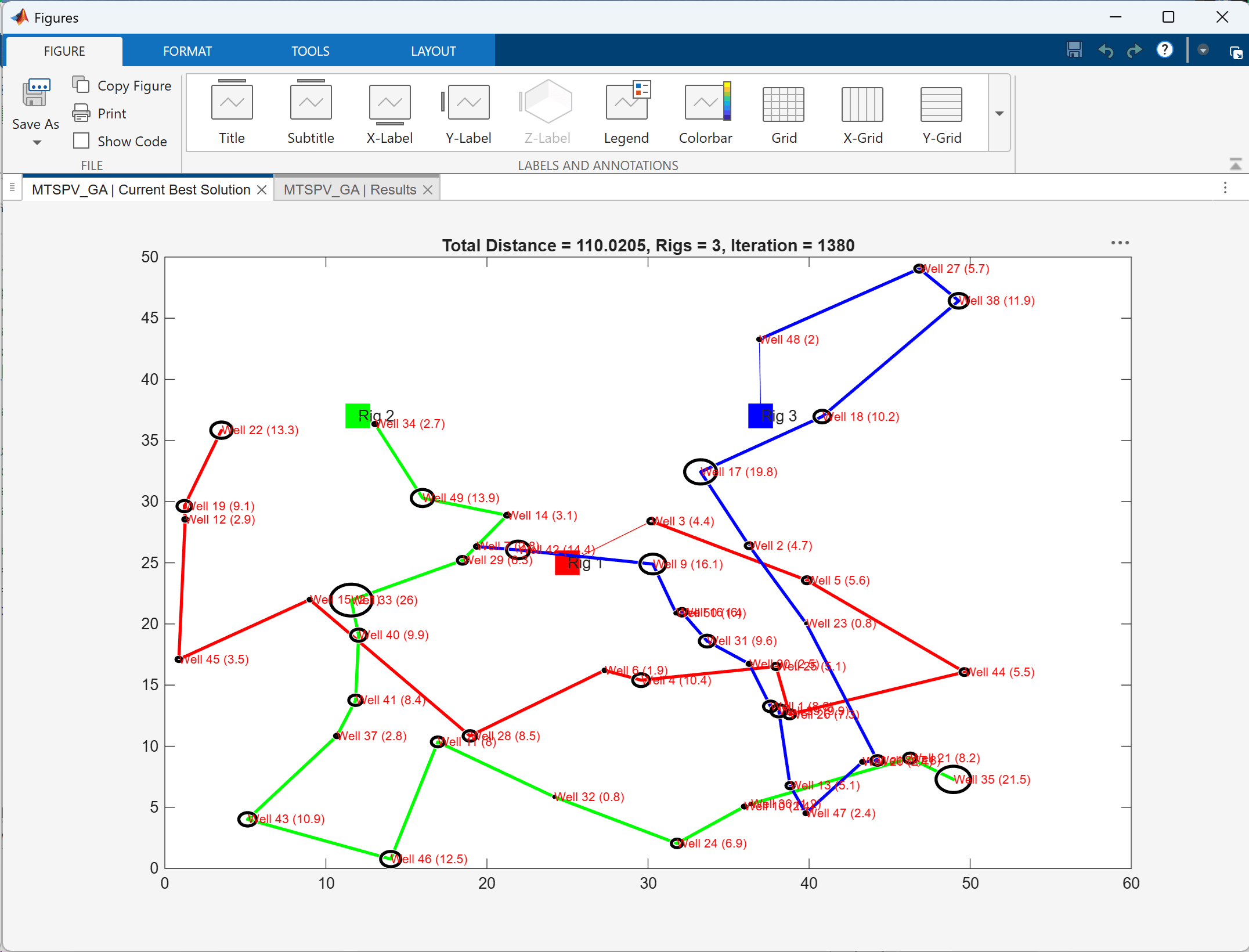
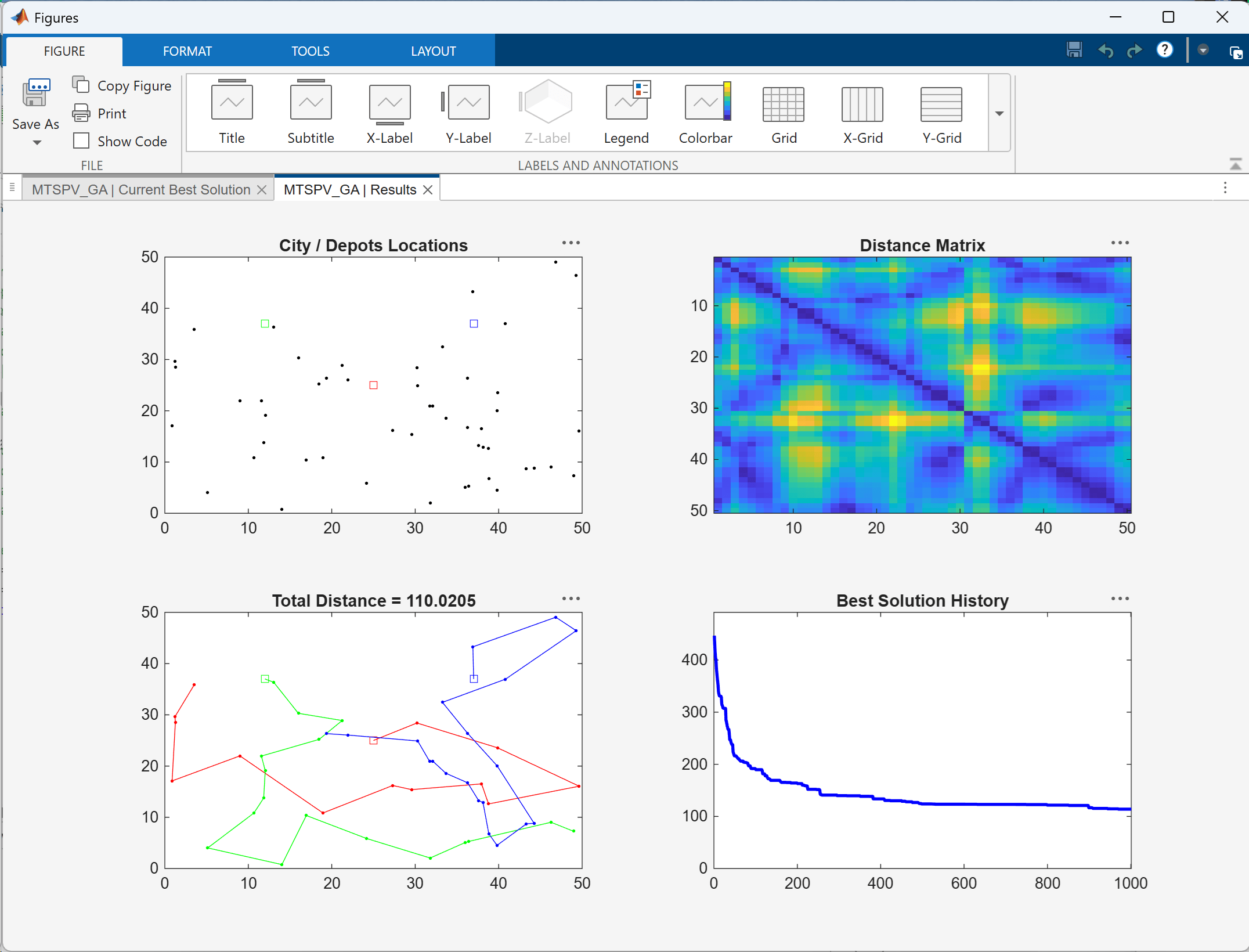
Schedules a fleet of drilling rigs across a field, each rig returning to its own depot: a multi-depot multiple travelling-salesman problem solved with a genetic algorithm. The petroleum-specific part is the objective: the distance matrix is weighted by each well’s drilling-priority and non-productive-time indices, so tours bend toward high-value wells instead of merely minimizing kilometres. Three rigs over roughly fifty wells converged from ~440 to a total weighted distance of 110.02 across 1,000 generations.
MATLAB Genetic Algorithm Multi-depot mTSP
Best-solution route map: three colour-coded rig tours over about fifty wells, each rig starting from its own depot marker, with every well labelled by its priority weight and drawn as a weight-scaled circle.
Best solution: three rig tours, markers scaled by well priority
Four-panel results view: well and depot locations, the weighted distance matrix as a heat map, the final rig tours, and the genetic algorithm's best-solution convergence curve over 1,000 iterations.
Results view: weighted distance matrix and GA convergence

02 · Computational Geometry

VoronoiAI2025

Weighted & segment Voronoi engine · desktop + WebAssembly

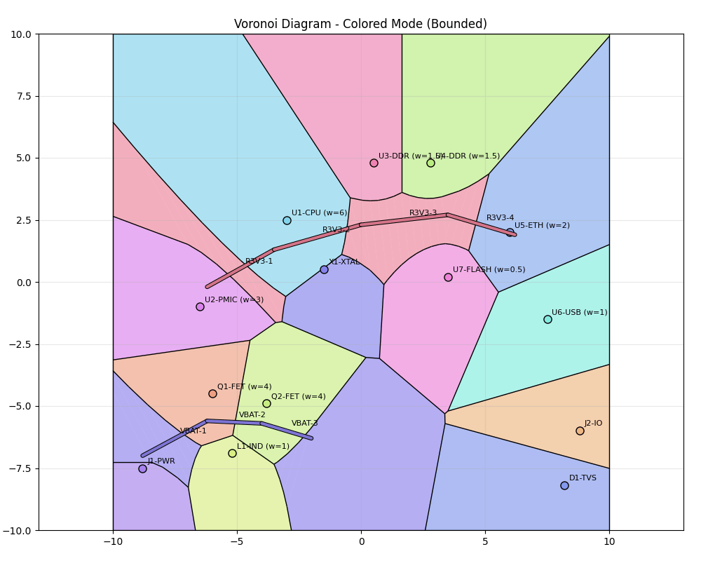
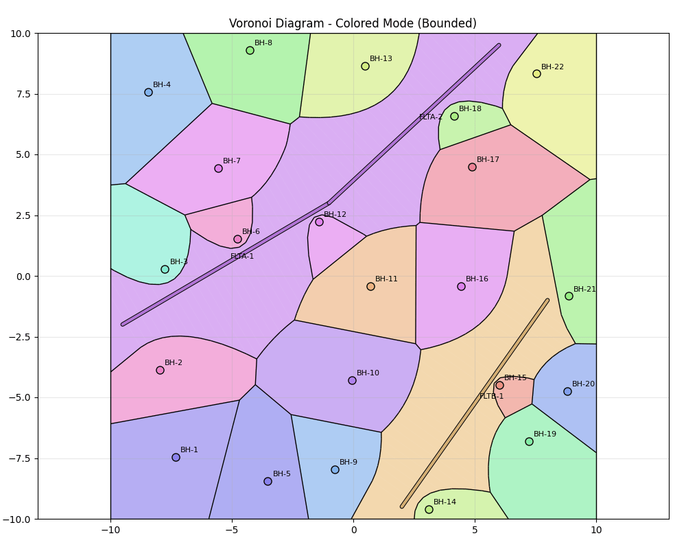
Models territory and drainage areas where a point is a well and a segment is a horizontal lateral. A “mirror-reflection” re-architecture made every cell a finite convex polygon, eliminating an entire class of infinite-region and degenerate-input bugs, then extended to power diagrams, exact parabolic-arc segment cells, and centroidal relaxation. One dependency-light core runs identically on the desktop and in the browser via Pyodide.

26 Engine invariants tested
11 Industry domains
1 core 2 platforms
Python scipy Pyodide / WASM Boost.Polygon Lloyd / CVT Tkinter
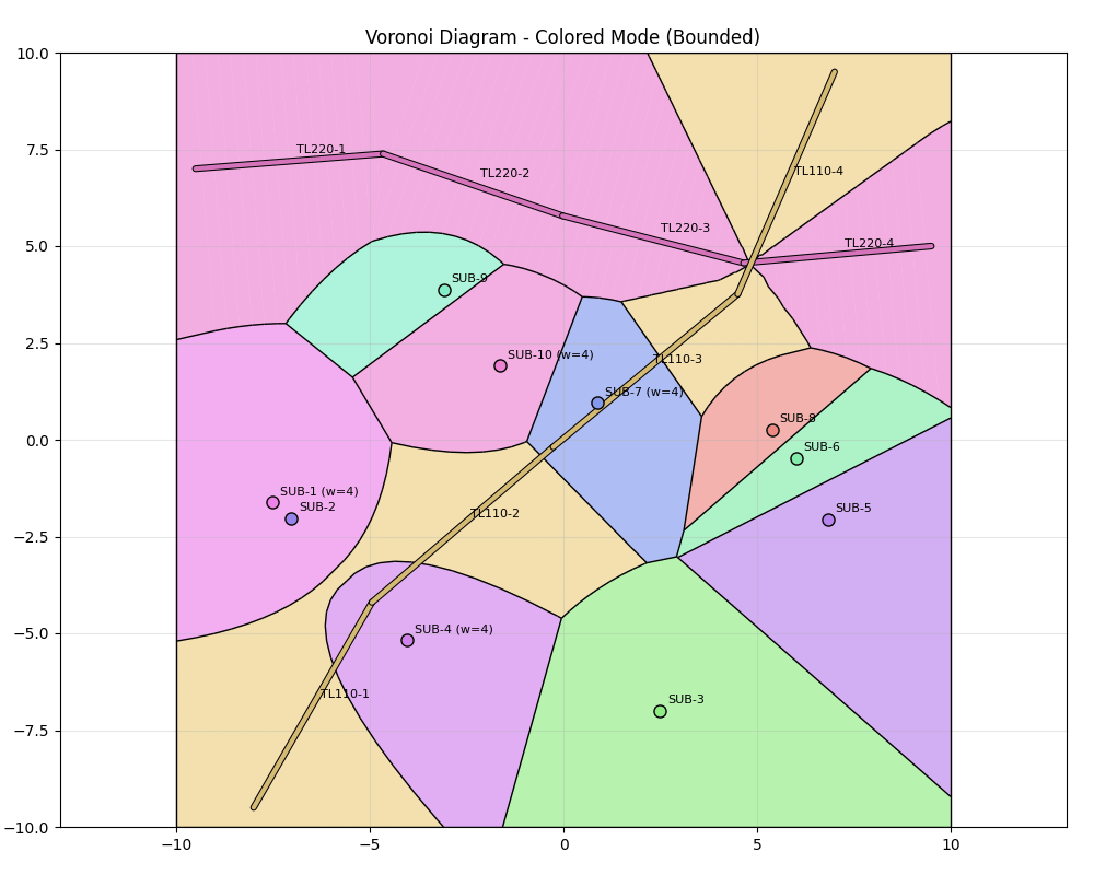
Voronoi drainage-area map of an oilfield: weighted vertical wells and horizontal laterals rendered as segments, each owning a coloured cell.
Oilfield drainage areas: weighted wells + horizontal laterals
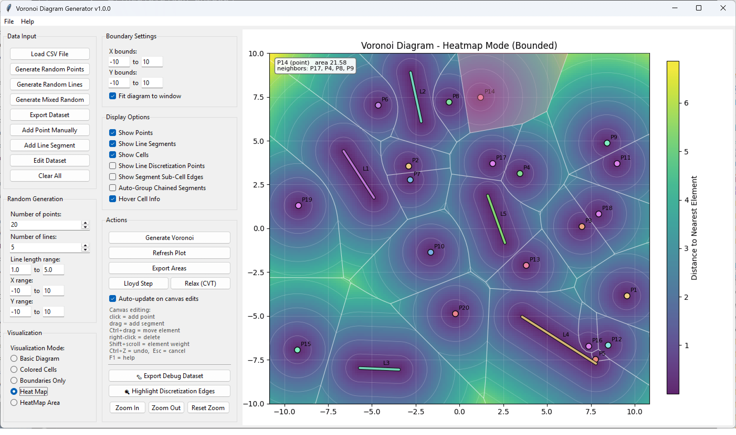
Voronoi Diagram Generator main window: panels for data input, boundary settings, display options, random generation and actions including Lloyd step and CVT relaxation, beside a bounded heat-map plot of twenty point seeds and five line segments shaded by distance to the nearest element, with a hover card reporting the cell under the cursor, its area and its neighbours.
The desktop application: distance heat map, live hover analytics, canvas editing
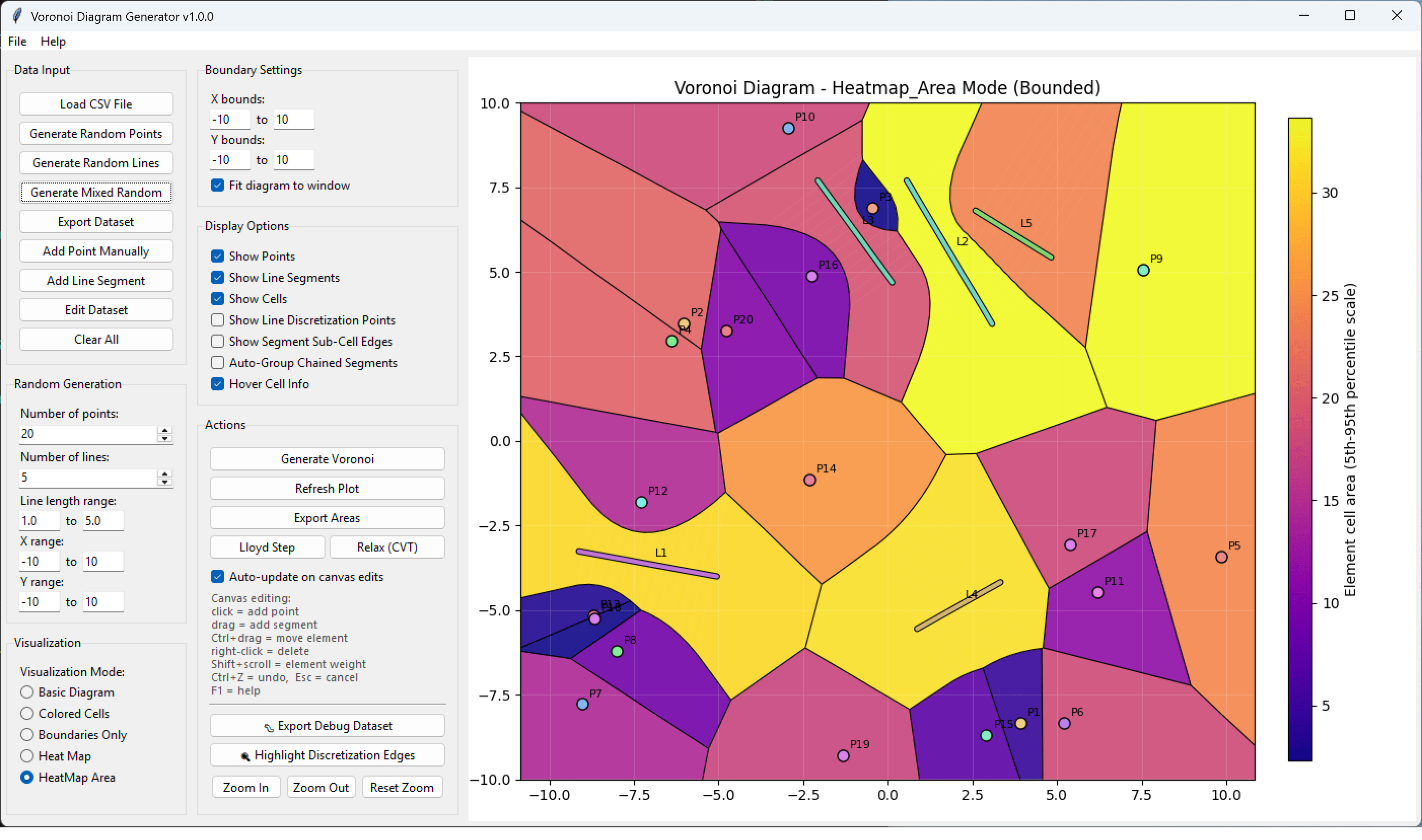
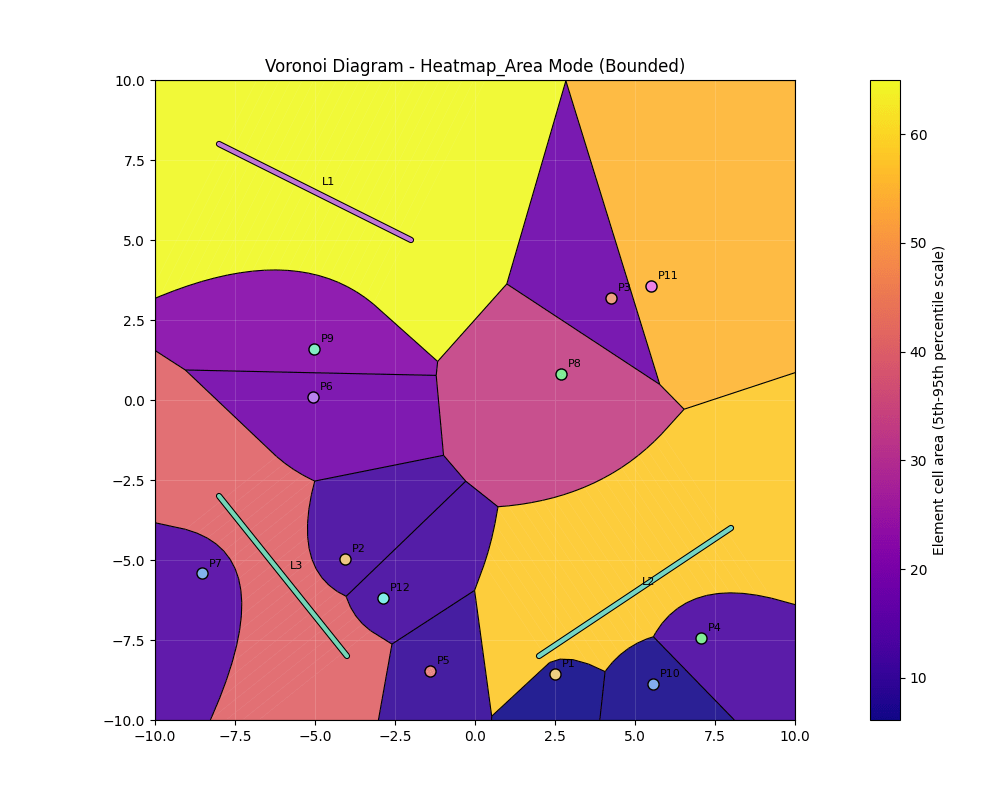
The same application in area heat-map mode: every cell shaded by its exact clipped area against a percentile colour scale, mixing point and line-segment seeds.
Area mode: cells shaded by exact clipped area
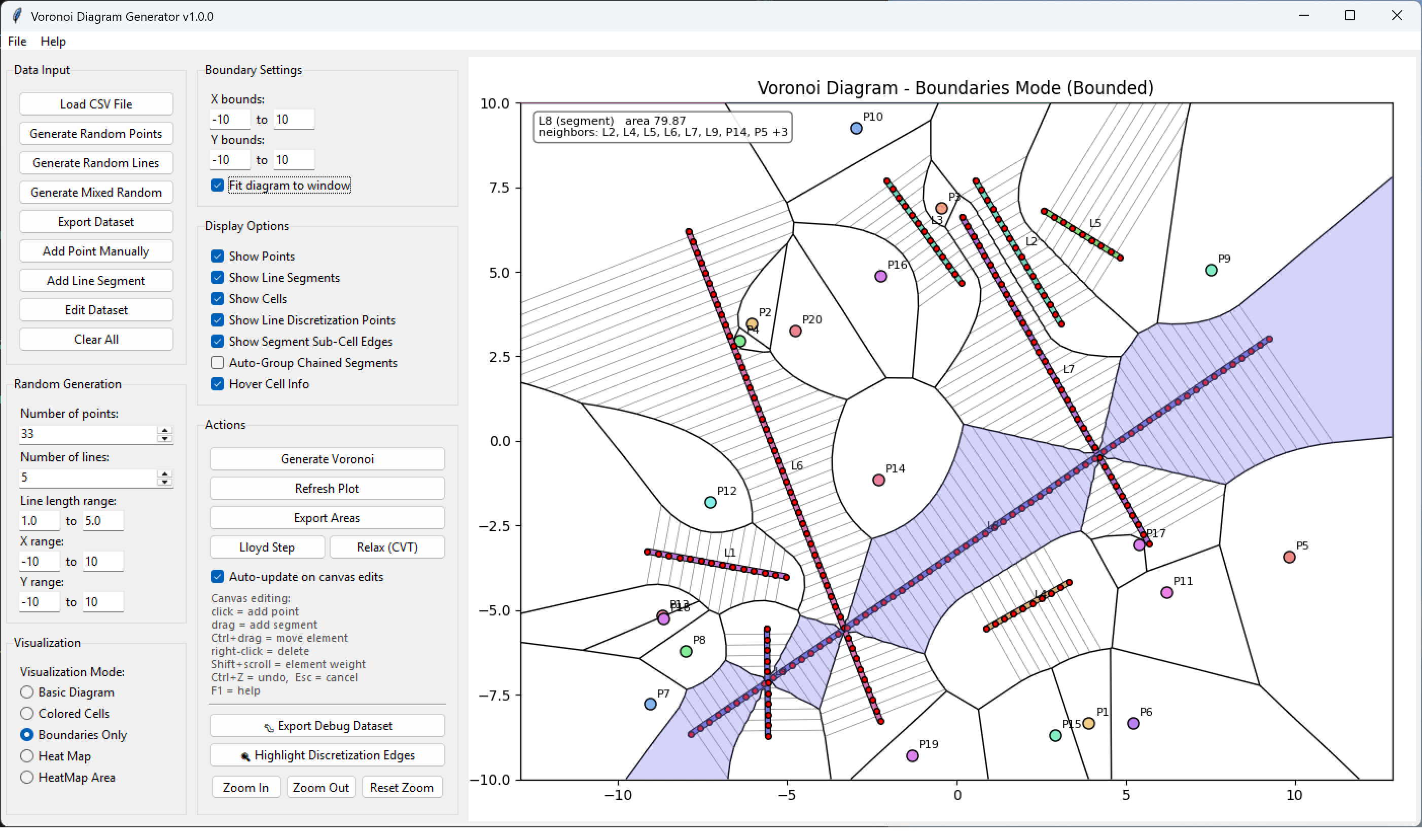
The same application in boundaries mode with line discretization points and segment sub-cell edges exposed, showing how a segment's cell is assembled, with a hover card reporting a segment cell's area and its eleven neighbours.
Boundaries mode: discretization points and segment sub-cell edges exposed
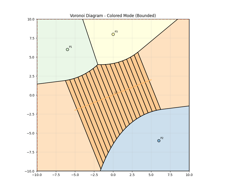
Prototype output showing striped, broken segment cells.
Before: prototype segment striping
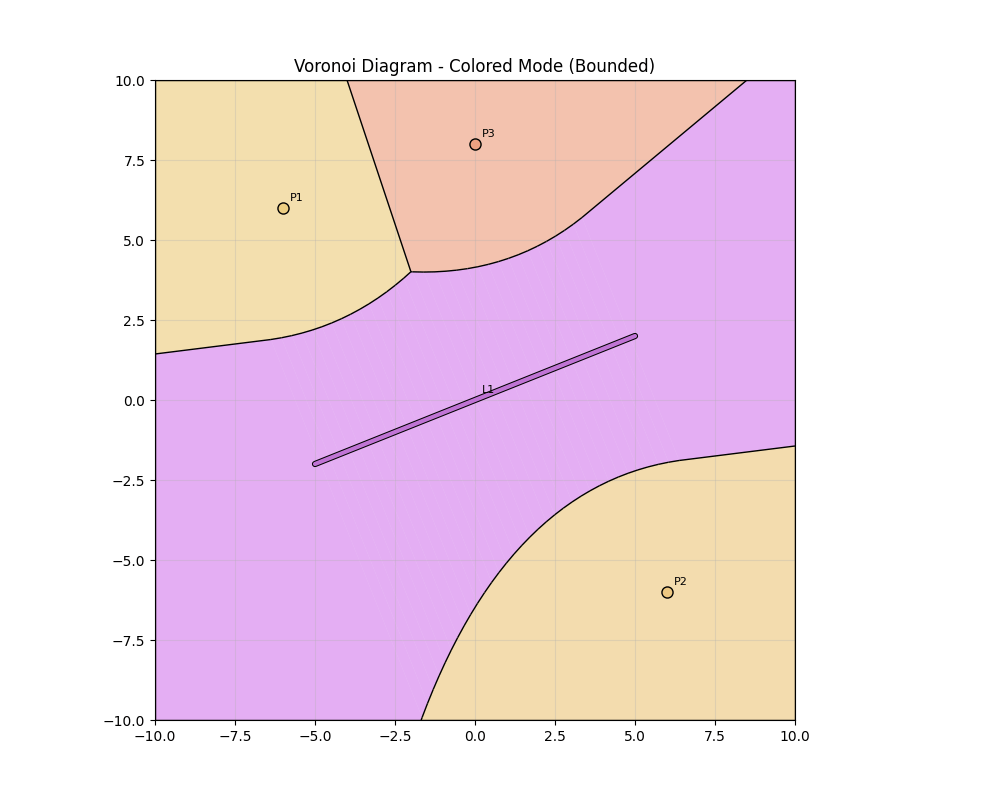
Rewritten output with clean merged segment cells.
After: merged segment cells
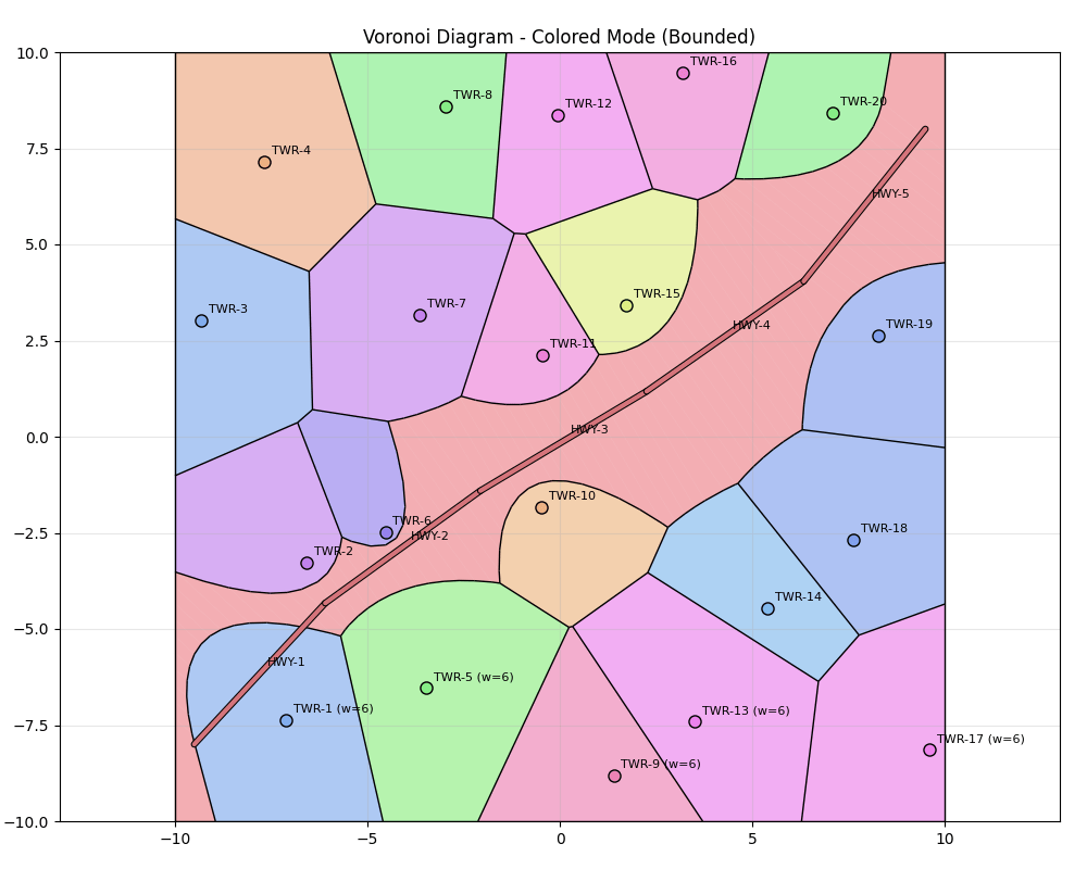
Power (weighted) Voronoi diagram where larger towers absorb more area.
Power diagram: weighted towers
Per-cell area heat map of a Voronoi tessellation.
Analytics: per-cell area heat map

Same engine, eleven industries: four shown
Power grid service territories.
Power gridsubstation territories
Telecom best-server coverage cells.
Telecombest-server coverage
PCB thermal zones rendered as a power diagram.
PCB thermalpower-weighted zones
Mining fault declustering polygons.
Miningfault declustering

03 · Waterflood Analytics

InterwellConnectivity

8-project .NET solution · OData service ↔ WinForms client

Quantifies which injector is feeding which producer across a mature waterflood, computing a well allocation factor for every injector–producer pair using an FIR capacitance model and a multivariate-regression alternative, both built on a custom matrix library. A genuine n-tier product: a WCF/OData service over Entity Framework, a rich client with a reusable interactive map control on an ArcGIS basemap, dedicated ETL and data-cleaning tools, and packaged MSI installers.
8 VS projects, one solution
2 Connectivity methods
n-tier Service · client · GIS
C# WCF / OData Entity Framework WinForms ArcGIS Server Math.NET
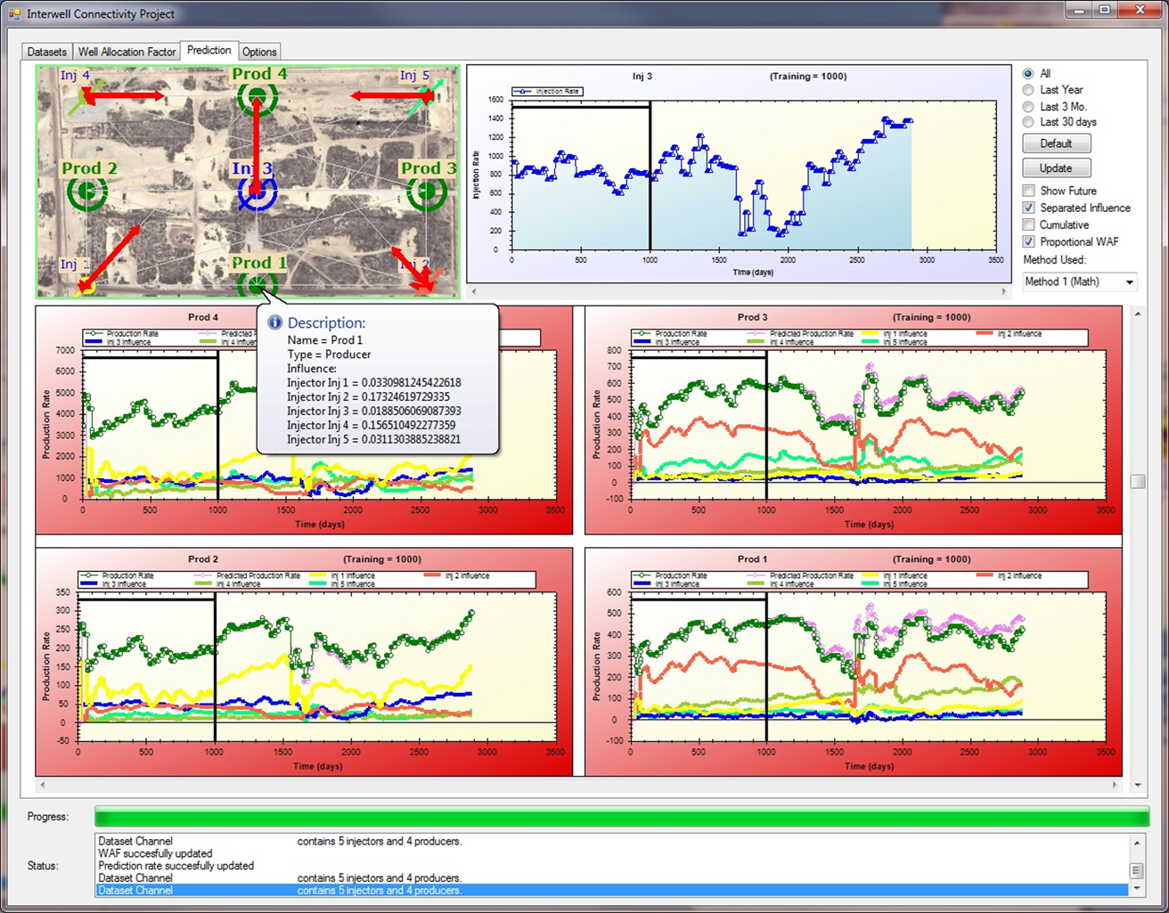
Interwell Connectivity prediction tab: a field map with five injectors and four producers linked by proportional influence arrows, an injection-rate history plot, and four per-producer panels overlaying measured production against the model prediction decomposed into each injector's contribution.
Prediction tab: per-producer influence decomposed by injector

04 · Production Forecasting

Decline Analysis

Sparse-data decline-curve analysis · VB.NET MDI + Python

Fits Arps decline curves to well production histories that report irregularly, then forecasts remaining recovery. Four models: classic exponential by closed-form logarithmic regression, plus exponential, harmonic and hyperbolic solved by handing the selected points to scipy’s differential evolution over a process boundary and reading back Qi, Di, b and R². The user picks the decline interval by clicking two points on the chart; events, stop and end dates are marked inline, and cumulative recovery is reported both analytically and trapezoidally.
4 Decline models fitted
2 DB engines · Access + SQL
6-step Schema-mapping wizard
VB.NET WinForms MDI Python · scipy ZedGraph Math.NET OLE DB / SQL Server
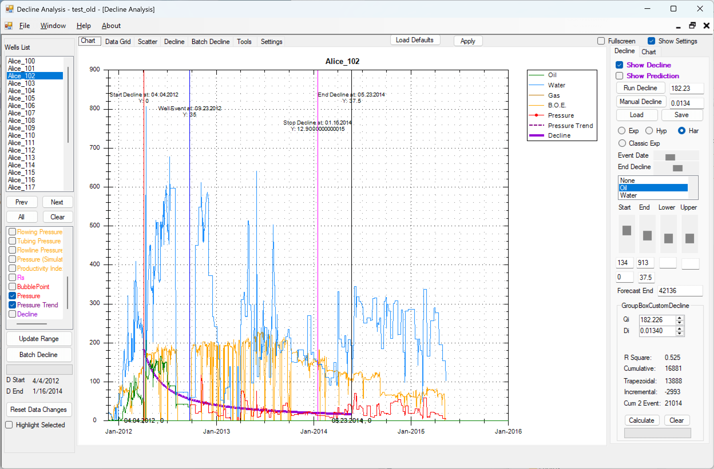
Decline Analysis main window: a well list, a multi-series production chart showing oil, water, gas, barrel-oil-equivalent and pressure against time with a fitted harmonic decline curve overlaid and the decline start, event, stop and end dates marked inline, and a results panel reporting the fitted initial rate, decline constant, R squared and cumulative recovery.
Harmonic fit over a sparse history: Qi 182.2, Di 0.0134, R² 0.525
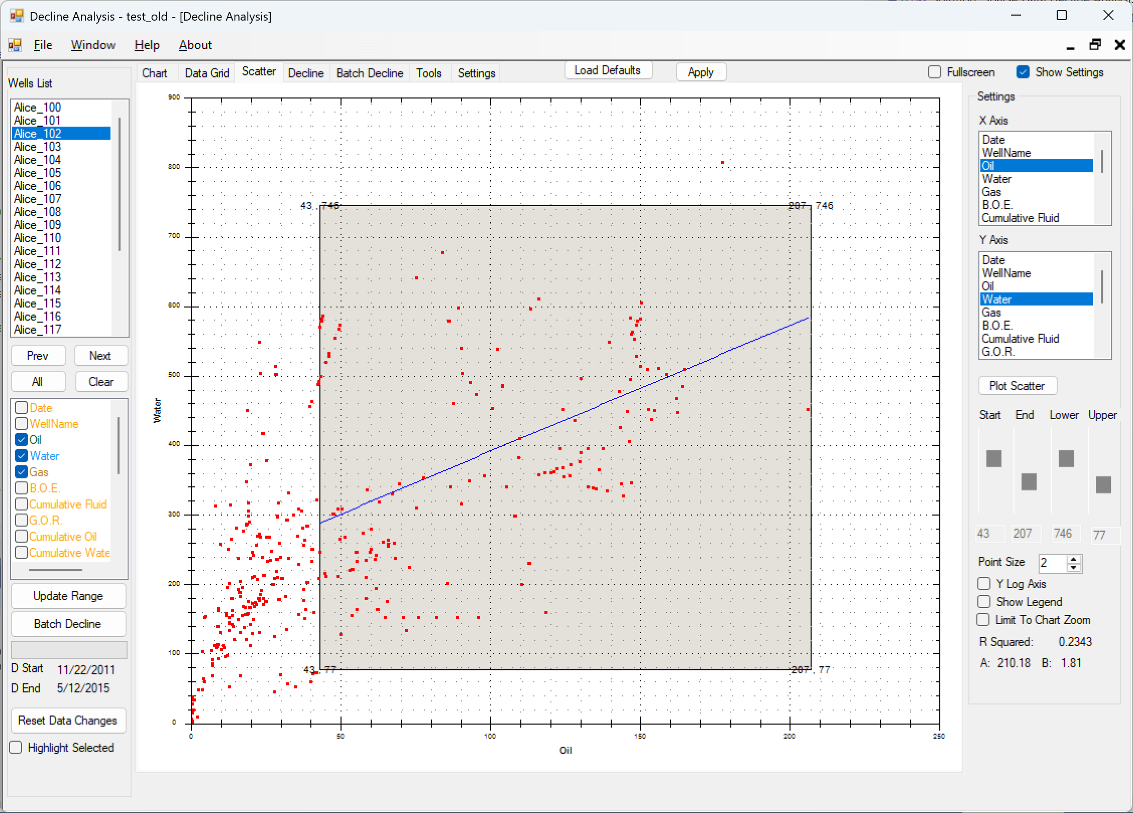
The scatter tab cross-plotting any two mapped production columns, here oil against water, with a box-selected subset of points regressed to a fitted line and its slope, intercept and R squared reported.
Scatter tab: cross-plot any two columns, regress a box-selected subset

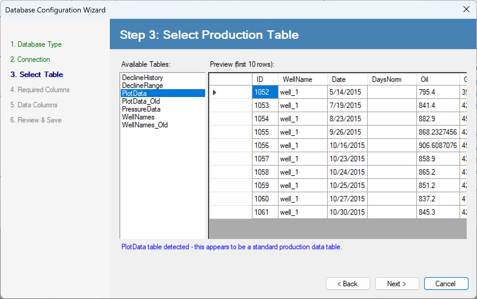
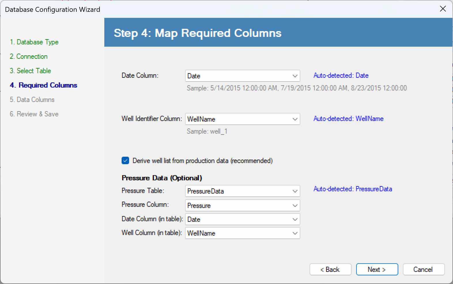
Pointed at any production database: a six-step mapping wizard
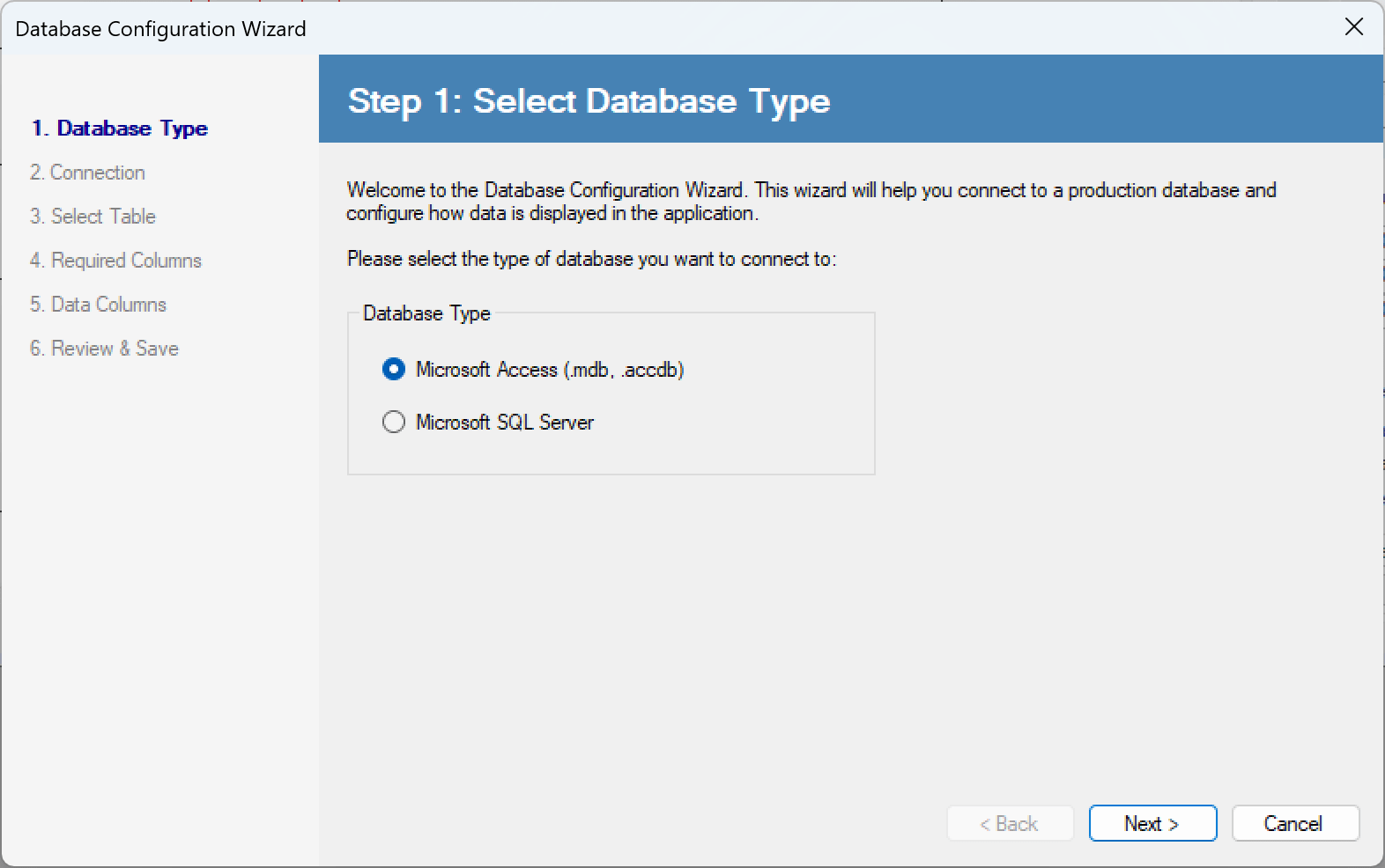
Wizard step one, choosing between a Microsoft Access file and a SQL Server connection.
Step 1: Access or SQL Server, behind one provider interface
Wizard step three listing the tables found in the database with a ten-row preview of the selected one, and a note reporting that a standard production data table was detected automatically.
Step 3: table discovery with preview and legacy-schema detection
Wizard step four mapping the date, well-identifier and optional pressure columns, each annotated with the value the application auto-detected.
Step 4: date, well and pressure columns auto-detected
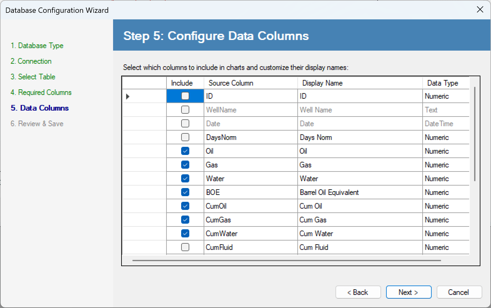
Wizard step five listing every candidate data column with an include checkbox, an editable display name and the detected data type.
Step 5: pick the curves, rename them, types inferred

The Rest of the Bench

Supporting tools from the same lab: petrophysics, soft computing, industry interoperability, and combinatorial optimization.
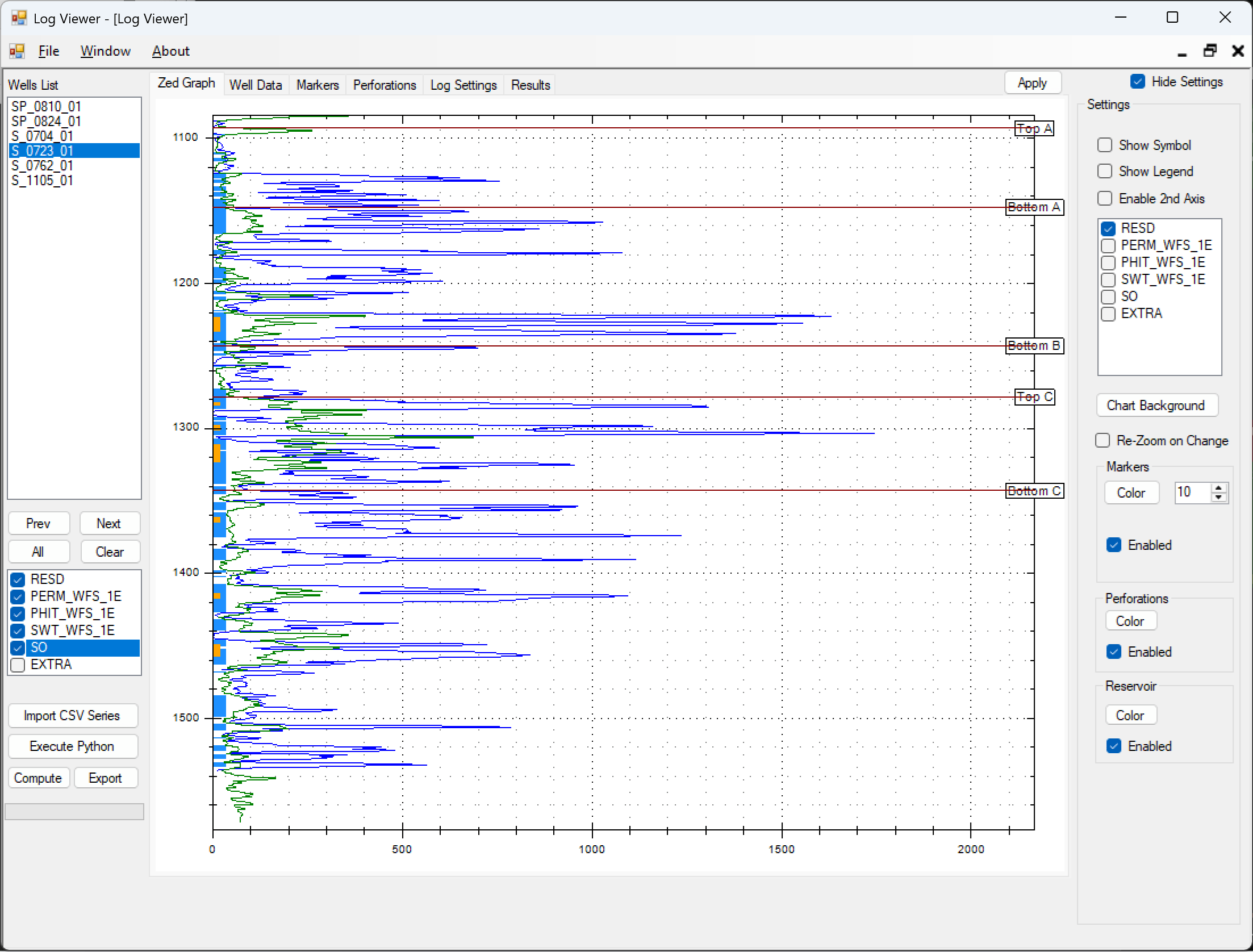
Log Viewer showing a multi-curve well-log depth plot with picked geological zone tops, a wells list, and a curve-selection settings panel.

Log Viewer

Petrophysics · VB.NET

MDI well-log viewer with custom-extended charting controls: multi-curve depth plots of porosity, permeability, saturation and resistivity, moving-average QC envelope bands, and interactive picking of geological zone tops and bottoms.

VB.NET WinForms ZedGraph

FuzzyNew

Soft computing · Python

Fuzzy-logic reservoir-quality scoring from geological inputs. Generalized the inference engine from hardcoded 3- and 4-input branches to arbitrary N inputs, and vectorized preprocessing for a ~100× speedup at roughly one-million-row scale.

Python scikit-fuzzy NumPy Tkinter

Petrel Workflow

Interoperability · VB.NET

Bridges Schlumberger Petrel property exports and the fuzzy reservoir model, streaming multi-million-row 3D grid files with column projection, then merging model results back into a Petrel-importable grid.

VB.NET CsvHelper Streaming I/O

Evolutionary Optimizer

Optimization · VB.NET

General-purpose real-coded genetic optimizer for any user-typed math expression, evaluated at runtime: tournament selection, crossover, per-gene mutation, elitism, and an immigration operator for population diversity.

VB.NET WinForms Runtime eval

Focus Areas

The kinds of problems the software lab took on.

  • 📈 Field-development optimization: deciding when to run every well under a shared facility constraint, solved three ways in parallel (mixed-integer programming, genetic algorithms, and greedy heuristics) so the fast method could be validated against the exact one.
  • 🧭 Computational geometry: Voronoi, power and segment diagrams for drainage and catchment areas, with centroidal relaxation and exact parabolic-arc cells, shipped to both desktop and the browser from a single code core.
  • 🛰️ Waterflood & production analytics: FIR capacitance and regression models quantifying injector–producer connectivity, delivered as a multi-tier .NET platform with a GIS map control over real production field data; plus decline-curve forecasting fitting exponential, harmonic and hyperbolic models to sparse histories by global optimization.
  • 🧪 Petrophysics & soft computing: fuzzy-logic reservoir-quality scoring, well-log interpretation and zone picking, and interoperability with industry-standard reservoir-modeling platforms such as Schlumberger Petrel.

Let’s Connect

More about my background and independent projects on the about page, or reach out directly.

USC CiSoft: Center for Interactive Smart Oilfield Technologies, a Chevron-funded research center at the USC Viterbi School of Engineering.
Every image on this page is a real rendered output from the tool described, not a mockup.